Navigation
- index
- modules |
- next |
- previous |
- Sage Tutorial, part 1.4 »

Here are some examples of calculus symbolic computations using Sage. They use the Maxima interface.
Work is being done to make the commands for the symbolic calculations given below more intuitive and natural. At the moment, we use the maxima class interface.
Consider an example of the motion of a certain spring-mass system that is modeled by the following differential equation subject to the initial conditions:
y'' +y' + 1.25 y = 3*cos(t), y(0) =2, y' (0) =3.
Its solution can be broken into sum of the transient y_c (t) and steady state solution U(t), where
y_c (t) = (22/17)*exp(-t/2)*cos(t) + (14/17)*exp(-t/2)*sin(t), U(t) = (12/17)*cos(t)+(48/17)*sin(t) .
We plot these functions using the following Sage commands.
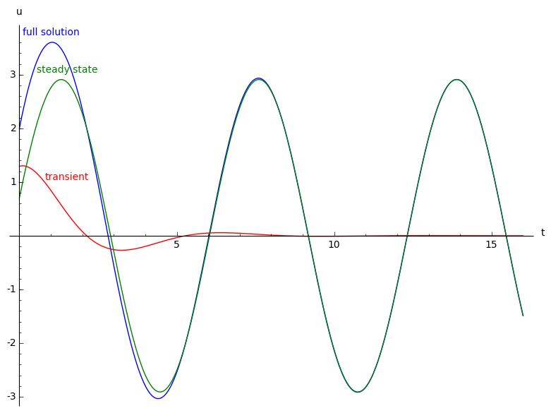
sage: u=((22/17)*e^(-x/2)*cos(x))+((14/17)*e^(-x/2)*sin(x))+((12/17)*cos(x))+((48/17)*sin(x))
sage: v=((22/17)*e^(-x/2)*cos(x))+((14/17)*e^(-x/2)*sin(x))
sage: y=((12/17)*cos(x))+((48/17)*sin(x))
sage: p1=plot(u,(x,0,16),axes_labels=['t','u'])
sage: p2=plot(v,(x,0,16),color='red')
sage: p3=plot(y,(x,0,16),color='green')
sage: a1=arrow((3,2), (1,1),color='red')
sage: plt=p1+p2+p3+a1
sage: plt+text('full solution',(1,3.8))+text('steady state',(1.5,3.1),color='green')+text('transient',(3.2,2.15),color='red')sage: p2=plot(v,(x,0,16),color='red')
y'' + 0.125*y' +y = 3*cos(0.3*t), y(0)=2, y'(0)=0.
We plot its solution along with with the forcing function using the following script.
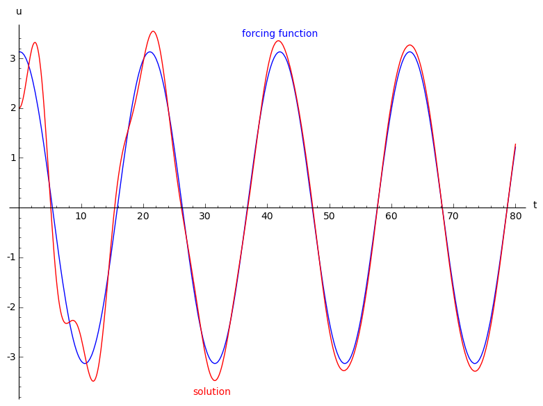
Similarly, we plot solutions to the following initial value problems:
y'' + 0.125*y' +y =3*cos(t), y(0)=2, y'(0) =0;
sage: u=3*cos(x-0.12533)
sage: v=((2)*e^(-0.0625*x)*cos(0.998045*x))+((-23.9218)*e^(-0.0625*x)*sin(0.998045*x))+((24)*sin(x))
sage: p1=plot(u,(x,0,60),axes_labels=['t','u'])
sage: p2=plot(v,(x,0,60),color='red')
sage: plt=p1+p2
sage: plt+text('forcing function',(6,-4.5))+text('solution',(8,10.7),color='red')
sage: #u=0.83205*cos(2*x-0.06934)
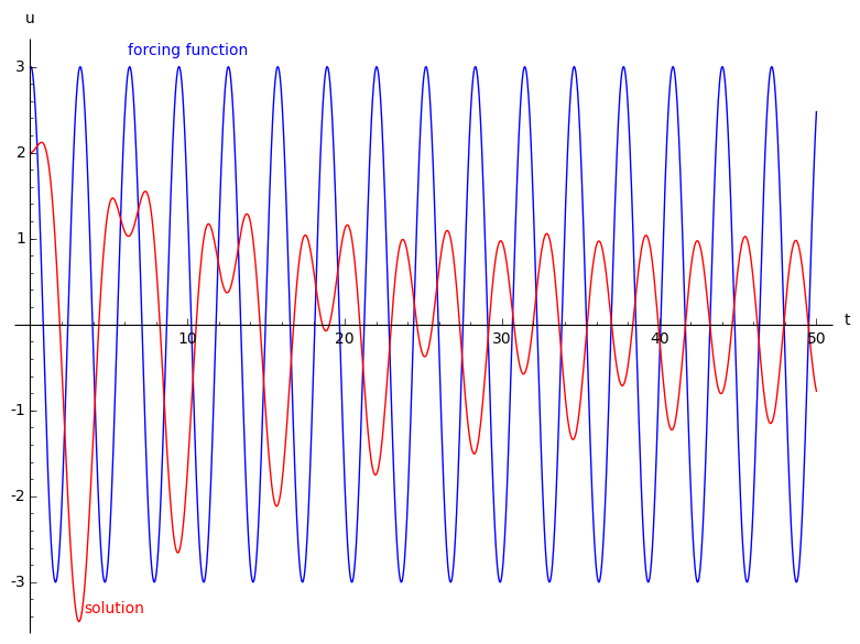
sage: u=3*cos(2*x-0.06934)
sage: v=((2.9931)*e^(-0.0625*x)*cos(0.998045*x))+((0.0215939)*e^(-0.0625*x)*sin(0.998045*x))+((0.0827586)*sin(2*x))+((-0.993103)*cos(2*x))
sage: p1=plot(u,(x,0,50),axes_labels=['t','u'])
sage: p2=plot(v,(x,0,50),color='red')
sage: plt=p1+p2
sage: plt+text('forcing function',(10,3.2))+text('solution',(5.3,-3.3),color='red')
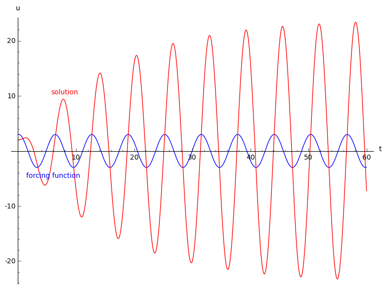
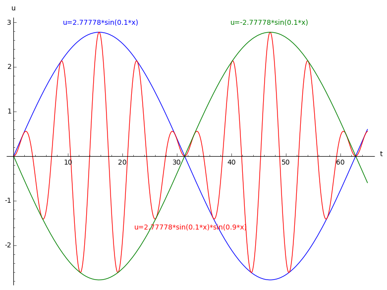
Now we consider the following initial value problems:
y'' + y =0.5*cos(0.8*t), y(0)=0, y'(0) =0;
sage: u1=2.77778*sin(0.1*x)
sage: u2=2.77778*sin(0.1*x)*sin(0.9*x)
sage: u3=-2.77778*sin(0.1*x)
sage: p1=plot(u1,(x,0,65),axes_labels=['t','u'])
sage: p2=plot(u2,(x,0,65),color='red')
sage: p3=plot(u3,(x,0,65),color='green')
sage: plt=p1+p2+p3
sage: plt+text('u=2.77778*sin(0.1*x)',(16,3))+text('u=2.77778*sin(0.1*x)*sin(0.9*x)',(32.5,-1.6),color='red')+text('u=-2.77778*sin(0.1*x)',(47,3),color='green')
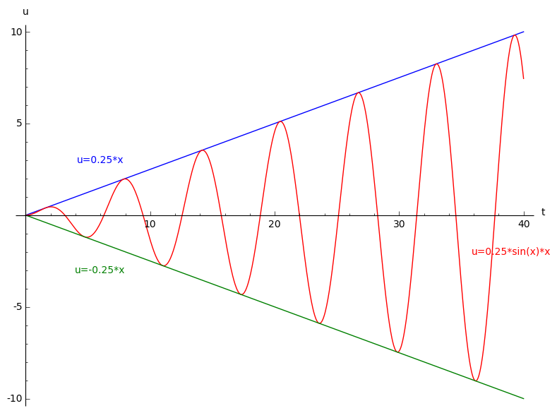
Finally, we plot solutions to the following initial value problem where resonance is observed:
y'' + y = 0.5*cos(t), y(0)=0, y'(0) =0;
sage: u1=0.25*x
sage: u2=0.25*sin(x)*x
sage: u3=-0.25*x
sage: p1=plot(u1,(x,0,40),axes_labels=['t','u'])
sage: p2=plot(u2,(x,0,40),color='red')
sage: p3=plot(u3,(x,0,40),color='green')
sage: plt=p1+p2+p3
sage: plt+text('u=0.25*x',(6,3))+text('u=0.25*sin(x)*x',(39,-2),color='red')+text('u=-0.25*x',(6,-3),color='green')
Differentiation:
sage: var('x k w')
(x, k, w)
sage: f = x^3 * e^(k*x) * sin(w*x); f
x^3*e^(k*x)*sin(w*x)
sage: f.diff(x)
w*x^3*cos(w*x)*e^(k*x) + k*x^3*e^(k*x)*sin(w*x) + 3*x^2*e^(k*x)*sin(w*x)
sage: latex(f.diff(x))
w x^{3} \cos\left(w x\right) e^{\left(k x\right)} + k x^{3} e^{\left(k x\right)} \sin\left(w x\right) + 3 \, x^{2} e^{\left(k x\right)} \sin\left(w x\right)
If you type view(f.diff(x)) another window will open up displaying the compiled output. In the notebook, you can enter
var('x k w')
f = x^3 * e^(k*x) * sin(w*x)
show(f)
show(f.diff(x))
into a cell and press shift-enter for a similar result. You can also differentiate and integrate using the commands
R = PolynomialRing(QQ,"x")
x = R.gen()
p = x^2 + 1
show(p.derivative())
show(p.integral())
in a notebook cell, or
sage: R = PolynomialRing(QQ,"x")
sage: x = R.gen()
sage: p = x^2 + 1
sage: p.derivative()
2*x
sage: p.integral()
1/3*x^3 + x
on the command line. At this point you can also type view(p.derivative()) or view(p.integral()) to open a new window with output typeset by LaTeX.
You can find critical points of a piecewise defined function:
sage: x = PolynomialRing(RationalField(), 'x').gen()
sage: f1 = x^0
sage: f2 = 1-x
sage: f3 = 2*x
sage: f4 = 10*x-x^2
sage: f = Piecewise([[(0,1),f1],[(1,2),f2],[(2,3),f3],[(3,10),f4]])
sage: f.critical_points()
[5.0]
Taylor series:
sage: var('f0 k x')
(f0, k, x)
sage: g = f0/sinh(k*x)^4
sage: g.taylor(x, 0, 3)
-62/945*f0*k^2*x^2 + 11/45*f0 - 2/3*f0/(k^2*x^2) + f0/(k^4*x^4)
sage: maxima(g).powerseries('_SAGE_VAR_x',0)    # TODO: write this without maxima
16*_SAGE_VAR_f0*('sum((2^(2*i1-1)-1)*bern(2*i1)*_SAGE_VAR_k^(2*i1-1)*_SAGE_VAR_x^(2*i1-1)/factorial(2*i1),i1,0,inf))^4
Of course, you can view the LaTeX-ed version of this using view(g.powerseries('x',0)).
The Maclaurin and power series of \(\log({\frac{\sin(x)}{x}})\):
sage: f = log(sin(x)/x)
sage: f.taylor(x, 0, 10)
-1/467775*x^10 - 1/37800*x^8 - 1/2835*x^6 - 1/180*x^4 - 1/6*x^2
sage: [bernoulli(2*i) for i in range(1,7)]
[1/6, -1/30, 1/42, -1/30, 5/66, -691/2730]
sage: maxima(f).powerseries(x,0)    # TODO: write this without maxima
'sum((-1)^i3*2^(2*i3-1)*bern(2*i3)*_SAGE_VAR_x^(2*i3)/(i3*factorial(2*i3)),i3,1,inf)
Numerical integration is discussed in Riemann and trapezoid sums for integrals below.
Sage can integrate some simple functions on its own:
sage: f = x^3
sage: f.integral(x)
1/4*x^4
sage: integral(x^3,x)
1/4*x^4
sage: f = x*sin(x^2)
sage: integral(f,x)
-1/2*cos(x^2)
Sage can also compute symbolic definite integrals involving limits.
sage: var('x, k, w')
(x, k, w)
sage: f = x^3 * e^(k*x) * sin(w*x)
sage: f.integrate(x)
((24*k^3*w - 24*k*w^3 - (k^6*w + 3*k^4*w^3 + 3*k^2*w^5 + w^7)*x^3 + 6*(k^5*w + 2*k^3*w^3 + k*w^5)*x^2 - 6*(3*k^4*w + 2*k^2*w^3 - w^5)*x)*cos(w*x)*e^(k*x) - (6*k^4 - 36*k^2*w^2 + 6*w^4 - (k^7 + 3*k^5*w^2 + 3*k^3*w^4 + k*w^6)*x^3 + 3*(k^6 + k^4*w^2 - k^2*w^4 - w^6)*x^2 - 6*(k^5 - 2*k^3*w^2 - 3*k*w^4)*x)*e^(k*x)*sin(w*x))/(k^8 + 4*k^6*w^2 + 6*k^4*w^4 + 4*k^2*w^6 + w^8)
sage: integrate(1/x^2, x, 1, infinity)
1
You can find the convolution of any piecewise defined function with another (off the domain of definition, they are assumed to be zero). Here is \(f\), \(f*f\), and \(f*f*f\), where \(f(x)=1\), \(0<x<1\):
sage: x = PolynomialRing(QQ, 'x').gen()
sage: f = Piecewise([[(0,1),1*x^0]])
sage: g = f.convolution(f)
sage: h = f.convolution(g)
sage: P = f.plot(); Q = g.plot(rgbcolor=(1,1,0)); R = h.plot(rgbcolor=(0,1,1))
To view this, type show(P+Q+R).
Regarding numerical approximation of \(\int_a^bf(x)\, dx\), where \(f\) is a piecewise defined function, can
sage: f1(x) = x^2
sage: f2(x) = 5-x^2
sage: f = Piecewise([[(0,1),f1],[(1,2),f2]])
sage: f.trapezoid(4)
Piecewise defined function with 4 parts, [[(0, 1/2), 1/2*x],
[(1/2, 1), 9/2*x - 2], [(1, 3/2), 1/2*x + 2],
[(3/2, 2), -7/2*x + 8]]
sage: f.riemann_sum_integral_approximation(6,mode="right")
19/6
sage: f.integral()
Piecewise defined function with 2 parts,
[[(0, 1), x |--> 1/3*x^3], [(1, 2), x |--> -1/3*x^3 + 5*x - 13/3]]
sage: f.integral(definite=True)
3
If you have a piecewise-defined polynomial function then there is a “native” command for computing Laplace transforms. This calls Maxima but it’s worth noting that Maxima cannot handle (using the direct interface illustrated in the last few examples) this type of computation.
sage: var('x s')
(x, s)
sage: f1(x) = 1
sage: f2(x) = 1-x
sage: f = Piecewise([[(0,1),f1],[(1,2),f2]])
sage: f.laplace(x, s)
-e^(-s)/s + (s + 1)*e^(-2*s)/s^2 + 1/s - e^(-s)/s^2
For other “reasonable” functions, Laplace transforms can be computed using the Maxima interface:
sage: var('k, s, t')
(k, s, t)
sage: f = 1/exp(k*t)
sage: f.laplace(t,s)
1/(k + s)
is one way to compute LT’s and
sage: var('s, t')
(s, t)
sage: f = t^5*exp(t)*sin(t)
sage: L = laplace(f, t, s); L
3840*(s - 1)^5/(s^2 - 2*s + 2)^6 - 3840*(s - 1)^3/(s^2 - 2*s + 2)^5 +
720*(s - 1)/(s^2 - 2*s + 2)^4
is another way.
Symbolically solving ODEs can be done using Sage interface with Maxima. See
sage:desolvers?
for available commands. Numerical solution of ODEs can be done using Sage interface with Octave (an experimental package), or routines in the GSL (Gnu Scientific Library).
An example, how to solve ODE’s symbolically in Sage using the Maxima interface (do not type the ...):
sage: y=function('y',x); desolve(diff(y,x,2) + 3*x == y, dvar = y, ics = [1,1,1])
3*x - 2*e^(x - 1)
sage: desolve(diff(y,x,2) + 3*x == y, dvar = y)
_K2*e^(-x) + _K1*e^x + 3*x
sage: desolve(diff(y,x) + 3*x == y, dvar = y)
(3*(x + 1)*e^(-x) + _C)*e^x
sage: desolve(diff(y,x) + 3*x == y, dvar = y, ics = [1,1]).expand()
3*x - 5*e^(x - 1) + 3

sage: f=function('f',x); desolve_laplace(diff(f,x,2) == 2*diff(f,x)-f, dvar = f, ics = [0,1,2])
x*e^x + e^x

sage: desolve_laplace(diff(f,x,2) == 2*diff(f,x)-f, dvar = f)
-x*e^x*f(0) + x*e^x*D[0](f)(0) + e^x*f(0)
If you have Octave and gnuplot installed,
sage: octave.de_system_plot(['x+y','x-y'], [1,-1], [0,2]) # optional - octave
yields the two plots \((t,x(t)), (t,y(t))\) on the same graph (the \(t\)-axis is the horizonal axis) of the system of ODEs
for \(0 <= t <= 2\). The same result can be obtained by using desolve_system_rk4:
sage: x, y, t = var('x y t')
sage: P=desolve_system_rk4([x+y, x-y], [x,y], ics=[0,1,-1], ivar=t, end_points=2)
sage: p1 = list_plot([[i,j] for i,j,k in P], plotjoined=True)
sage: p2 = list_plot([[i,k] for i,j,k in P], plotjoined=True, color='red')
sage: p1+p2
Graphics object consisting of 2 graphics primitives
Another way this system can be solved is to use the command desolve_system.
sage: t=var('t'); x=function('x',t); y=function('y',t)
sage: des = [diff(x,t) == x+y, diff(y,t) == x-y]
sage: desolve_system(des, [x,y], ics = [0, 1, -1])
[x(t) == cosh(sqrt(2)*t), y(t) == sqrt(2)*sinh(sqrt(2)*t) - cosh(sqrt(2)*t)]
The output of this command is not a pair of functions.
Finally, can solve linear DEs using power series:
sage: R.<t> = PowerSeriesRing(QQ, default_prec=10)
sage: a = 2 - 3*t + 4*t^2 + O(t^10)
sage: b = 3 - 4*t^2 + O(t^7)
sage: f = a.solve_linear_de(prec=5, b=b, f0=3/5)
sage: f
3/5 + 21/5*t + 33/10*t^2 - 38/15*t^3 + 11/24*t^4 + O(t^5)
sage: f.derivative() - a*f - b
O(t^4)
If \(f(x)\) is a piecewise-defined polynomial function on \(-L<x<L\) then the Fourier series
converges. In addition to computing the coefficients \(a_n,b_n\), it will also compute the partial sums (as a string), plot the partial sums (as a function of \(x\) over \((-L,L)\), for comparison with the plot of \(f(x)\) itself), compute the value of the FS at a point, and similar computations for the cosine series (if \(f(x)\) is even) and the sine series (if \(f(x)\) is odd). Also, it will plot the partial F.S. Cesaro mean sums (a “smoother” partial sum illustrating how the Gibbs phenomenon is mollified).
sage: f1 = lambda x: -1
sage: f2 = lambda x: 2
sage: f = Piecewise([[(0,pi/2),f1],[(pi/2,pi),f2]])
sage: f.fourier_series_cosine_coefficient(5,pi)
-3/5/pi
sage: f.fourier_series_sine_coefficient(2,pi)
-3/pi
sage: f.fourier_series_partial_sum(3,pi)
-3*cos(x)/pi - 3*sin(2*x)/pi + sin(x)/pi + 1/4
Type show(f.plot_fourier_series_partial_sum(15,pi,-5,5)) and show(f.plot_fourier_series_partial_sum_cesaro(15,pi,-5,5)) (and be patient) to view the partial sums.