Navigation
- index
- modules |
- next |
- previous |
- Sage Tutorial, part 1.1 »

Numerical computation has been one of the most
central applications of the computer since its invention. In modern
society, the significance of the speed and effectiveness of the computational algorithms has only increased with applications in data analysis,
information retrieval, optimization and simulation.
Most numerical algorithms are implemented in a variety of programming languages. There are various commercial collections of software
libraries with numerical analysis functionality, mostly written in Fortran, C and C++. These include, among others, the IMSL and NAG
libraries. Computer algebra systems and applications developed specially for numerical computing include MATLAB, S-PLUS, Mathematica, Maple, IDL and LabVIEW. There are also free and open source alternatives such as the GNU Scientific Library (GSL), R, Scilab, Freemat,
and Sage.
Many computer algebra systems (e.g., Maple, Mathematica, and
MuPad within MATLAB) contain an implementation of a new programming language
specific to that system. In contrast, Sage uses Python, which is a popular and widespread high-level programming language. The Python
language is considered simple and easy to learn while making the use
of more advanced programming techniques, such as object-oriented programming and defining new methods and data types, possible in the
study of the mathematics. Python functions as a common user interface to Sage's nearly one hundred software packages.
Some of the advantages of Sage in scientific programming are the
free availability of the source code and openness of development. Most
commercial software do not have their algorithms publicly available,
which makes it impossible to revise and audit the functionality of the
code. Therefore the use of the built-in functions of these programs
may be inadequate in some mathematical studies that are based on the
results given by these algorithms. This is not the case in open source
software, where the user can verify the individual implementations of
the algorithms.
In many situations, the Python interpreter is fast enough for common calculations. However, sometimes considerable speed is needed in
numerical computations. Sage supports Cython, which is a compiled
language based on Python that supports calling C functions and declaring C types on variables and class attributes. It is used for writing fast
Python extension modules and interfacing Python with C libraries.
Significant parts of the NumPy and SciPy libraries included with Sage
are written in Cython. In addition, techniques like distributed computing and parallel processing using multi-core processors or multiple
processors are supported in Sage.
Sage includes the Matplotlib library for plotting two-dimensional
objects. For three-dimensional plotting, Sage has Jmol, an open-source
Java viewer. Additionally, the Tachyon 3D raytracer may be used for
more detailed plotting. Sage's
interact
function can also bring added
value to the study of numerical methods by introducing controllers
that allow dynamical adjusting of the parameters in a Sage program.
Python is a popular multipurpose programming language. When
augmented with special libraries/modules, it is suitable also for scientific computing and visualization. These modules make scientific
computing with Python similar to what commercial packages such as
MATLAB, Mathematica, and Maple offer. Special Python libraries
like NumPy, SciPy and CVXOPT allow fast machine precision floating
point computations and provide subroutines to all basic numerical analysis functions. As such the Python language can be used to combine
several software components. For data visualization there are numer-
ous Python based libraries such as Matplotlib. There is a very wide
collection of external libraries. These packages/libraries are available
either for free or under permissive open source licenses which makes
these very attractive for university level teaching purposes.
The mission of the Sage project is to bring a large number of program
libraries under the principle of the GNU General Public License under
the same umbrella. Sage offers a common interface for all its components and its command language is Python. Originally developed for
the purposes of number theory and algebraic geometry, it presently
supports more than 100 special libraries. Augmented with these, Sage
is able to carry out both symbolic and numeric computing.
NumPy provides support for fast multi-dimensional arrays and numerous matrix operations. The syntax of NumPy resembles the syntax
of MATLAB in many ways. NumPy includes subpackages for linear
algebra, discrete Fourier transforms and random number generators,
among others. The SciPy library is a library of scientific tools for
Python. It uses the array object of the NumPy library as its basic
data structure. SciPy contains various high level scientific modules
for linear algebra, numerical integration, optimizing, image processing,
ODE solvers and signal processing, et cetera.
CVXOPT is a library specialized in optimization. It extends the
built-in Python objects with dense and sparse matrix object types.
CVXOPT contains methods for both linear and nonlinear convex op-
timization. For statistical computing and graphics, Sage supports the
R environment, which can be used via the Sage Notebook. Some statistical features are also provided in SciPy, but not as comprehensively
as in R.
Computing the solution of some given equation is one of the fundamental problems of numerical analysis. If a real-valued function is differentiable and the derivative is known, then Newton's method may be used to find an approximation to its roots. In Newton's method, an initial guess x_0 for a root of the differentiable function f: R -> R is made. The consecutive iterative steps are defined by
x_{k+1} = x_k - f(x_k) / f' f(x_k) , k=0,1,2,3,\ldots
f(x_n -h) f(x_n+h)<0
In order to avoid an infinite loop, the maximum number of iterations is limited by the parameter maxn
sage: def newton_method(f, c, maxn, h):
f(x) = f
iterates = [c]
j = 1
while True:
c = c - f(c)/derivative(f(x))(x=c)
iterates.append(c)
if f(c-h)*f(c+h) < 0 or j == maxn:
break
j += 1
return c, iterate
sage: f(x) = x^2-3
h = 10^-5
initial = 2.0
maxn = 10
z, iterates = newton_method(f, initial, maxn, h/2.0)
print "Root =", z
Numerical integration methods can prove useful if the integrand is known only at certain points or the antiderivate is very difficult or even mpossible to find. In education, calculating numerical methods by hand may be useful in some cases, but computer programs are usually better suited in finding patterns and comparing different methods. In the next example, three numerical integration methods are implemented in Sage: the midpoint rule, the trapezoidal rule and Simpson's rule. The differences between the exact value of integration and the approximation are tabulated by the number of subintervals n
sage: f(x) = x^2-3
sage: a = 0.0
sage: b = 2.0
sage: table = []
sage: exact = integrate(f(x), x, a, b)
sage: for n in [4, 10, 20, 50, 100]:
....:     h = (b-a)/n
....:     midpoint = sum([f(a+(i+1/2)*h)*h for i in range(n)])
....:     trapezoid = h/2*(f(a) + 2*sum([f(a+i*h) for i in range(1,n)])
....:     + f(b))
....:     simpson = h/3*(f(a) + sum([4*f(a+i*h) for i in range(1,n,2)])
....:     + sum([2*f(a+i*h) for i in range (2,n,2)]) + f(b))
....:     table.append([n, h.n(digits=2), (midpoint-exact).n(digits=6),
....:     (trapezoid-exact).n(digits=6), (simpson-exact).n(digits=6)])
....:     html.table(table, header=["n", "h", "Midpoint rule",
....:     "Trapezoidal rule", "Simpson's rule"])
There are also built-in methods for numerical integration in Sage.
For instance, it is possible to automatically produce piecewise-defined
line functions defined by the trapezoidal rule or the midpoint rule.
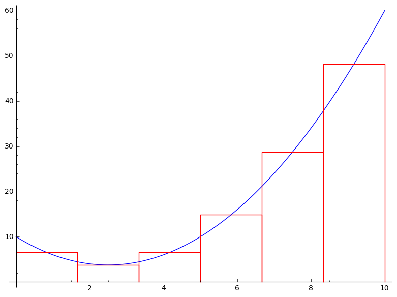
These functions can be used to visualize different geometric interpretations of the numerical integration methods. In the next example,
midpoint rule is used to calculate an approximation for the definite
integral of the function
f(x) =x^2 -5x + 10
over the interval [0;10] using six subintervals
sage: f(x) = x^2-5*x+10
sage: f = Piecewise([[(0,10), f]])
sage: g = f.riemann_sum(6, mode="midpoint")
sage: F = f.plot(color="blue")
sage: R = add([line([[a,0],[a,f(x=a)],[b,f(x=b)],[b,0]], color="red") for (a,b), f in g.list()]
sage: show(F+R)
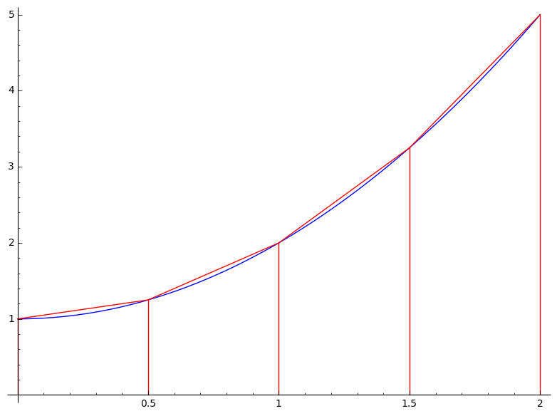
The Trapezoid Rule approximates the area under a given curve by finding the area under a linear approximation to the curve. The linear segments are given by the secant lines through the endpoints of the subintervals: for f(x)=x^2+1 on [0,2] with 4 subintervals, this looks like:
sage: x = var('x')
sage: f1(x) = x^2 + 1
sage: f = Piecewise([[(0,2),f1]])
sage: trapezoid_sum = f.trapezoid(4)
sage: P = f.plot(rgbcolor=(0,0,1), plot_points=40)
sage: Q = trapezoid_sum.plot(rgbcolor=(1,0,0), plot_points=40)
sage: L = add([line([[a,0],[a,f(x=a)]], rgbcolor=(1,0,0)) for (a,b), f in trapezoid_sum.list()])
sage: M = line([[2,0],[2,f1(2)]], rgbcolor=(1,0,0))
sage: show(P + Q + L + M)
To integrate the function cos(2*x)^4 +sin(x) we do
sage: numerical_integral(lambda x: cos(2*x)^5 + sin(x),  0, 2*pi)
(2.3561944901923457, 5.322071926740605e-14)
The input can be any callable:
sage: numerical_integral(lambda x: cos(2*x)^5 + sin(x),  0, 2*pi)
(2.3561944901923457, 5.322071926740605e-14)
We check this with a symbolic integration:
sage: (cos(2*x)^4+sin(x)).integral(x,0,2*pi)
3/4*pi
It is possible to integrate on infinite intervals as well by using +Infinity or -Infinity in the interval argument. For example:
sage: f = exp(-2*x)
sage: numerical_integral(f, 0, +Infinity)
(0.4999999999993456, 2.5048509541974486e-07)
We can also numerically integrate symbolic expressions using either this function (which uses GSL) or the native integration (which uses Maxima):
sage: (x^3*sin(1/x)).nintegral(x,0,pi)
(9.874626194990983, 6.585622218041451e-08, 315, 0)
Regarding numerical approximation of \(\int_a^bf(x)\, dx\), where \(f\) is a piecewise defined function, can
sage: f1(x) = x^2
sage: f2(x) = 5-x^2
sage: f = Piecewise([[(0,1),f1],[(1,2),f2]])
sage: f.trapezoid(4)
Piecewise defined function with 4 parts, [[(0, 1/2), 1/2*x],
[(1/2, 1), 9/2*x - 2], [(1, 3/2), 1/2*x + 2],
[(3/2, 2), -7/2*x + 8]]
sage: f.riemann_sum_integral_approximation(6,mode="right")
19/6
sage: f.integral()
Piecewise defined function with 2 parts,
[[(0, 1), x |--> 1/3*x^3], [(1, 2), x |--> -1/3*x^3 + 5*x - 13/3]]
sage: f.integral(definite=True)
3
Differentiation:
sage: var('x k w')
(x, k, w)
sage: f = x^3 * e^(k*x) * sin(w*x); f
x^3*e^(k*x)*sin(w*x)
sage: f.diff(x)
w*x^3*cos(w*x)*e^(k*x) + k*x^3*e^(k*x)*sin(w*x) + 3*x^2*e^(k*x)*sin(w*x)
sage: latex(f.diff(x))
w x^{3} \cos\left(w x\right) e^{\left(k x\right)} + k x^{3} e^{\left(k x\right)} \sin\left(w x\right) + 3 \, x^{2} e^{\left(k x\right)} \sin\left(w x\right)
If you type view(f.diff(x)) another window will open up displaying the compiled output. In the notebook, you can enter
var('x k w')
f = x^3 * e^(k*x) * sin(w*x)
show(f)
show(f.diff(x))
into a cell and press shift-enter for a similar result. You can also differentiate and integrate using the commands
R = PolynomialRing(QQ,"x")
x = R.gen()
p = x^2 + 1
show(p.derivative())
show(p.integral())
in a notebook cell, or
sage: R = PolynomialRing(QQ,"x")
sage: x = R.gen()
sage: p = x^2 + 1
sage: p.derivative()
2*x
sage: p.integral()
1/3*x^3 + x
on the command line. At this point you can also type view(p.derivative()) or view(p.integral()) to open a new window with output typeset by LaTeX.
You can find critical points of a piecewise defined function:
sage: x = PolynomialRing(RationalField(), 'x').gen()
sage: f1 = x^0
sage: f2 = 1-x
sage: f3 = 2*x
sage: f4 = 10*x-x^2
sage: f = Piecewise([[(0,1),f1],[(1,2),f2],[(2,3),f3],[(3,10),f4]])
sage: f.critical_points()
[5.0]
Taylor series:
sage: var('f0 k x')
(f0, k, x)
sage: g = f0/sinh(k*x)^4
sage: g.taylor(x, 0, 3)
-62/945*f0*k^2*x^2 + 11/45*f0 - 2/3*f0/(k^2*x^2) + f0/(k^4*x^4)
sage: maxima(g).powerseries('_SAGE_VAR_x',0)    # TODO: write this without maxima
16*_SAGE_VAR_f0*('sum((2^(2*i1-1)-1)*bern(2*i1)*_SAGE_VAR_k^(2*i1-1)*_SAGE_VAR_x^(2*i1-1)/factorial(2*i1),i1,0,inf))^4
Of course, you can view the LaTeX-ed version of this using view(g.powerseries('x',0)).
The Maclaurin and power series of \(\log({\frac{\sin(x)}{x}})\):
sage: f = log(sin(x)/x)
sage: f.taylor(x, 0, 10)
-1/467775*x^10 - 1/37800*x^8 - 1/2835*x^6 - 1/180*x^4 - 1/6*x^2
sage: [bernoulli(2*i) for i in range(1,7)]
[1/6, -1/30, 1/42, -1/30, 5/66, -691/2730]
sage: maxima(f).powerseries(x,0)    # TODO: write this without maxima
'sum((-1)^i3*2^(2*i3-1)*bern(2*i3)*_SAGE_VAR_x^(2*i3)/(i3*factorial(2*i3)),i3,1,inf)
Numerical integration is discussed in Riemann and trapezoid sums for integrals below.
Sage can integrate some simple functions on its own:
sage: f = x^3
sage: f.integral(x)
1/4*x^4
sage: integral(x^3,x)
1/4*x^4
sage: f = x*sin(x^2)
sage: integral(f,x)
-1/2*cos(x^2)
Sage can also compute symbolic definite integrals involving limits.
sage: var('x, k, w')
(x, k, w)
sage: f = x^3 * e^(k*x) * sin(w*x)
sage: f.integrate(x)
((24*k^3*w - 24*k*w^3 - (k^6*w + 3*k^4*w^3 + 3*k^2*w^5 + w^7)*x^3 + 6*(k^5*w + 2*k^3*w^3 + k*w^5)*x^2 - 6*(3*k^4*w + 2*k^2*w^3 - w^5)*x)*cos(w*x)*e^(k*x) - (6*k^4 - 36*k^2*w^2 + 6*w^4 - (k^7 + 3*k^5*w^2 + 3*k^3*w^4 + k*w^6)*x^3 + 3*(k^6 + k^4*w^2 - k^2*w^4 - w^6)*x^2 - 6*(k^5 - 2*k^3*w^2 - 3*k*w^4)*x)*e^(k*x)*sin(w*x))/(k^8 + 4*k^6*w^2 + 6*k^4*w^4 + 4*k^2*w^6 + w^8)
sage: integrate(1/x^2, x, 1, infinity)
1
You can find the convolution of any piecewise defined function with another (off the domain of definition, they are assumed to be zero). Here is \(f\), \(f*f\), and \(f*f*f\), where \(f(x)=1\), \(0<x<1\):
sage: x = PolynomialRing(QQ, 'x').gen()
sage: f = Piecewise([[(0,1),1*x^0]])
sage: g = f.convolution(f)
sage: h = f.convolution(g)
sage: P = f.plot(); Q = g.plot(rgbcolor=(1,1,0)); R = h.plot(rgbcolor=(0,1,1))
To view this, type show(P+Q+R).
If you have a piecewise-defined polynomial function then there is a “native” command for computing Laplace transforms. This calls Maxima but it’s worth noting that Maxima cannot handle (using the direct interface illustrated in the last few examples) this type of computation.
sage: var('x s')
(x, s)
sage: f1(x) = 1
sage: f2(x) = 1-x
sage: f = Piecewise([[(0,1),f1],[(1,2),f2]])
sage: f.laplace(x, s)
-e^(-s)/s + (s + 1)*e^(-2*s)/s^2 + 1/s - e^(-s)/s^2
For other “reasonable” functions, Laplace transforms can be computed using the Maxima interface:
sage: var('k, s, t')
(k, s, t)
sage: f = 1/exp(k*t)
sage: f.laplace(t,s)
1/(k + s)
is one way to compute LT’s and
sage: var('s, t')
(s, t)
sage: f = t^5*exp(t)*sin(t)
sage: L = laplace(f, t, s); L
3840*(s - 1)^5/(s^2 - 2*s + 2)^6 - 3840*(s - 1)^3/(s^2 - 2*s + 2)^5 +
720*(s - 1)/(s^2 - 2*s + 2)^4
is another way.
Symbolically solving ODEs can be done using Sage interface with Maxima. See
sage:desolvers?
for available commands. Numerical solution of ODEs can be done using Sage interface with Octave (an experimental package), or routines in the GSL (Gnu Scientific Library).
An example, how to solve ODE’s symbolically in Sage using the Maxima interface (do not type the ...):
sage: y=function('y',x); desolve(diff(y,x,2) + 3*x == y, dvar = y, ics = [1,1,1])
3*x - 2*e^(x - 1)
sage: desolve(diff(y,x,2) + 3*x == y, dvar = y)
_K2*e^(-x) + _K1*e^x + 3*x
sage: desolve(diff(y,x) + 3*x == y, dvar = y)
(3*(x + 1)*e^(-x) + _C)*e^x
sage: desolve(diff(y,x) + 3*x == y, dvar = y, ics = [1,1]).expand()
3*x - 5*e^(x - 1) + 3

sage: f=function('f',x); desolve_laplace(diff(f,x,2) == 2*diff(f,x)-f, dvar = f, ics = [0,1,2])
x*e^x + e^x

sage: desolve_laplace(diff(f,x,2) == 2*diff(f,x)-f, dvar = f)
-x*e^x*f(0) + x*e^x*D[0](f)(0) + e^x*f(0)
If you have Octave and gnuplot installed,
sage: octave.de_system_plot(['x+y','x-y'], [1,-1], [0,2]) # optional - octave
yields the two plots \((t,x(t)), (t,y(t))\) on the same graph (the \(t\)-axis is the horizonal axis) of the system of ODEs
for \(0 <= t <= 2\). The same result can be obtained by using desolve_system_rk4:
sage: x, y, t = var('x y t')
sage: P=desolve_system_rk4([x+y, x-y], [x,y], ics=[0,1,-1], ivar=t, end_points=2)
sage: p1 = list_plot([[i,j] for i,j,k in P], plotjoined=True)
sage: p2 = list_plot([[i,k] for i,j,k in P], plotjoined=True, color='red')
sage: p1+p2
Graphics object consisting of 2 graphics primitives
Another way this system can be solved is to use the command desolve_system.
sage: t=var('t'); x=function('x',t); y=function('y',t)
sage: des = [diff(x,t) == x+y, diff(y,t) == x-y]
sage: desolve_system(des, [x,y], ics = [0, 1, -1])
[x(t) == cosh(sqrt(2)*t), y(t) == sqrt(2)*sinh(sqrt(2)*t) - cosh(sqrt(2)*t)]
The output of this command is not a pair of functions.
Finally, can solve linear DEs using power series:
sage: R.<t> = PowerSeriesRing(QQ, default_prec=10)
sage: a = 2 - 3*t + 4*t^2 + O(t^10)
sage: b = 3 - 4*t^2 + O(t^7)
sage: f = a.solve_linear_de(prec=5, b=b, f0=3/5)
sage: f
3/5 + 21/5*t + 33/10*t^2 - 38/15*t^3 + 11/24*t^4 + O(t^5)
sage: f.derivative() - a*f - b
O(t^4)
If \(f(x)\) is a piecewise-defined polynomial function on \(-L<x<L\) then the Fourier series
converges. In addition to computing the coefficients \(a_n,b_n\), it will also compute the partial sums (as a string), plot the partial sums (as a function of \( x\) over \((-L,L)\), for comparison with the plot of \( f(x)\) itself), compute the value of the FS at a point, and similar computations for the cosine series (if \( f(x)\) is even) and the sine series (if \(f(x)\) is odd). Also, it will plot the partial F.S. Cesaro mean sums (a “smoother” partial sum illustrating how the Gibbs phenomenon is mollified).
sage: f1 = lambda x: -1
sage: f2 = lambda x: 2
sage: f = Piecewise([[(0,pi/2),f1],[(pi/2,pi),f2]])
sage: f.fourier_series_cosine_coefficient(5,pi)
-3/5/pi
sage: f.fourier_series_sine_coefficient(2,pi)
-3/pi
sage: f.fourier_series_partial_sum(3,pi)
-3*cos(x)/pi - 3*sin(2*x)/pi + sin(x)/pi + 1/4
Type show(f.plot_fourier_series_partial_sum(15,pi,-5,5)) and show(f.plot_fourier_series_partial_sum_cesaro(15,pi,-5,5)) (and be patient) to view the partial sums.