Heaviside FunctionBrown University, Applied Mathematics |
Continuous, Piecewise, and Piecewise Continuous
It is a good idea to review the idea of how we can define 3 different kinds of functions. We are all familiar with the idea of a Continuous Function. For example, we could say:
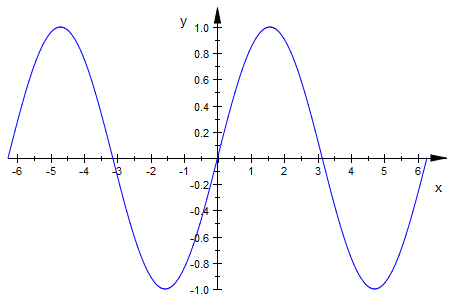
For all x, $f(x) = \sin(x)$ or equivilantly in mathematical jargon $\forall x, x \in \Re, f(x)= sin(x)$
and this would define our continuous function. Most of the time, we just write $f(x)=\sin(x)$ and it is assumed that our function is continuous, unless specified. You will recall that defining a continuous function in MuPAD is quite easy. MuPAD will assume that it will be defined for all X, unless otherwise specified:
reset()
f(x) := sin(x)
![]()
plot(f(x),x=-2*PI..2*PI)
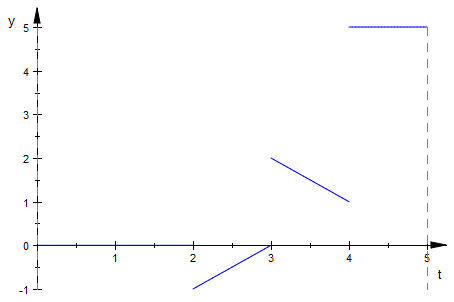
Now we will consider Piecewise Functions. What is different? You may remember from high school that a piecewise function is a collection of slices of continuous functions, defined on a given interval. For this function to be "continuous piecewise", we will need our function to be defined at all points in our given interval. It is rare that you would encounter a function that is piecewise but not piecewise continuous, but it is still a valid consideration. Note that the interval for a piecewise function can be infinite, but most functions will be on a finite interval. Below we will see how define a piecewise function in MuPAD:
f(t):=piecewise([0<=t<=2,0],[2<=t<=3,t-3],[3<=t<=4,5-t],[4<=t<=5,5])
![piecewise([t in Dom::Interval([0], [2]), 0], [t in Dom::Interval([2], [3]), t - 3], [t in Dom::Interval([3], [4]), 5 - t], [t in Dom::Interval([4], [5]), 5])](images10/image3.png)
plot(f(t),t=0..5)
Heaviside Step Function
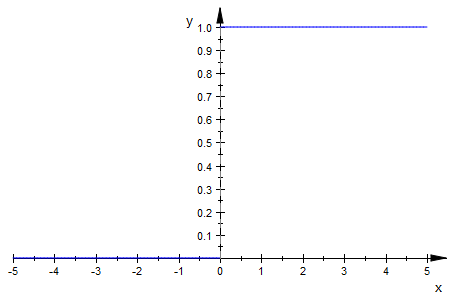
The heaviside function is a very simple piecewise function, defined on an infinite interval $(-\infty,\infty)$. It is denoted as H(t) and historically the function will only use the independent variable "t", because it is used to model physical systems in real time. With that said, the function has the value 0 for all negative values of t, and is the value 1 for all positive values of t. The most interesting part of this function is its value at 0. The value is the average of the limits from the left and the right as H(t) approaches 0, which is 1/2. Visualizing the function in MuPAD will help you understand what the function looks like.
To define the heaviside function, we will simply type the following code, which should seem straightforward:
heaviside(x)
![]()
plot(%)
heaviside(-4)
![]()
heaviside(0)
![]()
heaviside(19)
![]()
Shifting Heaviside
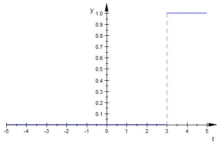
We can also shift the Heaviside function along the X axis. By applying a condition within the parenthesis of the H(t) function, we can accomplish this, creating a shifted Heaviside function. For example $H(t-3)$ would slide the function to the right 3 units. We can also use 2 Heaviside functions to create an interval where the function is the value 1, and zero outside this interval. The way to do this is to create the difference of two shifted Heaviside functions. The following MuPAD code will illustrate these properties:
heaviside(t-3)
![]()
plot(%)
heaviside(t-3)-heaviside(t-5)
![]()
plot(%, t=0..7)
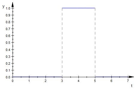
In general, to create a Heaviside interval of this type we will use the following formula:
$H(t-a)-H(t-b)$ will define the interval $[a,b]$ and remain 0 outside this interval.
Application of Heaviside to Continuous and Piecewise Continuous Functions
Why is the Heaviside function so important? We will use this function when using the Laplace transform to perform several tasks, such as shifting functions, and making sure that our function is defined for t > 0. Think about what would happen if we multiplied a regular H(t) function to a normal function, say sin(t). When t > 0, the function will remain the same. When t = 0, the function will be half of its normal value. When t < 0, the function will be identically 0. What about when we multiply a heaviside interval and a regular function. The function will be half of its normal value on the endpoints of the interval, its regular value within the interval, and identically zero outside this interval. This is a very good model of real life physical functions. Most functions in real life are piecewise continuous. For example, consider a dark room. The lights are off, so the amount of electricity running through the light-bulb circuit is 0. When you turn on the lights, your alternating current (modeled as a sine curve) suddenly appears in time. When you turn on another light, or appliance using electricity, your function will jump to different valued functions. When you eventually turn off all your electronics and the lights, the function returns to zero. You have just created a piecewise continuous function in time. By using intervals of the Heaviside function, we can model many different kinds of scenarios, such as the one we just described. The following MuPAD code will illustrate this concept:
When multiplying functions by heaviside functions in MuPAD, we will want to assume t > 0
assume(t>0)
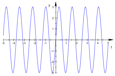
g(t) := 3*sin(5*t)
![]()
plot(%)
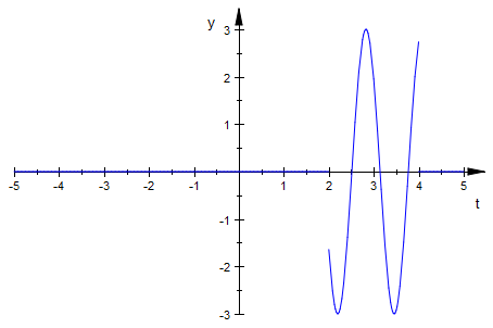
p(t):=g(t)*(heaviside(t-2)-heaviside(t-4))
![]()
plot(%)
f(t):=piecewise([0<=t<=2,0],[2<=t<=3,t-3],[3<=t<=4,3*sin(5*t)],[4<=t<=5,5])
![piecewise([t in Dom::Interval([0], [2]), 0], [t in Dom::Interval([2], [3]), t - 3], [t in Dom::Interval([3], [4]), 3*sin(5*t)], [t in Dom::Interval([4], [5]), 5])](images10/image14.png)
plot(f(t),t=0..6)
assume(t>0)
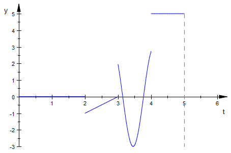
f2(t):=(t-3)*(heaviside(t-2)-heaviside(t-3))+(3*sin(5*t))*(heaviside(t-3)-heaviside(t-4))+5*(heaviside(t-4)-heaviside(t-5))
![]()
plot(f2(t), t=-1..6)
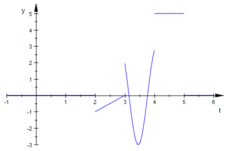
Notice that our function is now defined for all t, and anyhwere t < 0, we are returned the value 0 for y
MuPAD can even simplify our anwer:
f3(t):=simplify(f2(t))
![]()
Example. Find the Laplace transform of the following piecewise function using the MuPAD Laplace Solver:
g(x) := piecewise([0<=x<=3, 0], [3<=x<=7, x-7], [7<=x<=9, 9-x], [9<=x<=12, 15])
First, assume that x is greater than 0:
assume(x>0)
g2(x) := (x-7)*(heaviside(x-3)-heaviside(x-7)) + (9-x)*(heaviside(x-7)-heaviside(x-9)) + 15*(heaviside(x-9)-heaviside(x-12))
g3(x) := simplify(g2(x))
Finally, apply MuPAD's Laplace command and put in terms of lambda for final answer:
L(g) := laplace(g3(x),x,`λ`)
+ \frac{e^{-9\lambda} \left( 2\,\lambda \,e^{2\lambda} - e^{2\lambda}
+1 \right)}{\lambda^2} -
\frac{e^{-7\lambda} \left( 4\,\lambda \,e^{4\lambda} - e^{4\lambda} +1 \right)}{\lambda^2} . \]
Example. Compute the inverse Laplace transform of the piecewise function in problem 3:
inverse_L(g) := ilaplace((15*exp(-9*`λ`)/`λ`) - (15*exp(-12*`λ`)/`λ`) + (2*`λ`*exp(-7*`λ`) - exp(-7*`λ`) + exp(-9*`λ`))/(`λ`)^2 - (4*`λ`*exp(-3*`λ`) - exp(-3*`λ`) + exp(-7*`λ`))/(`λ`)^2,`λ`,t)
Note: check that the inverse Laplace transform is correct by taking the Laplace transform of the result:
laplace(inverse_L(g),t,`λ`)
Note 2: The form of this new Laplace transform may look a bit different from the solution to problem 3, but the answers are equivalent!
Home |
< Previous |
Next > |