Global Eigensolvers
Unlike local eigensolvers global methods for eigenproblems do not require a good initial guess for an eigenvalue. In addition, they provide the entire eigenspectrum. We will discuss two such approaches that are based on two different concepts: The QR method and the Lanczos method. The first one is general and the second] one is appropriate for symmetric sparse systems.
The QR Eigensolver
The main idea of this method is to construct a
sequence of similar matrices
![]() ,
where
,
where
![]() and
and ![]() approaches an upper triangular matrix as
approaches an upper triangular matrix as
![]() of the form
of the form
![\begin{displaymath}A_k \rightarrow \left [ \begin{array}{ccccccccc}
\lambda_1 & ...
...\vdots\\
& & & \ddots \\
& & & &\lambda_n
\end{array}\right ]\end{displaymath}](img5.gif)
The Schur triangulization theorem [#!Golub-vanLoan!#]
guarantees that this triangular matrix exists if an orthonormal
matrix ![]() is involved in the similarity transformation.
The scalar entries in the diagonal correspond to real eigenvalues.
However, for non-symmetric matrices we may encounter complex eigenvalues,
which manifest themselves as
is involved in the similarity transformation.
The scalar entries in the diagonal correspond to real eigenvalues.
However, for non-symmetric matrices we may encounter complex eigenvalues,
which manifest themselves as
![]() submatrices on the diagonal
in the form
submatrices on the diagonal
in the form
![\begin{displaymath}A_k\rightarrow \left [ \begin{array}{ccccccccccc}
\lambda _1 ...
...& & & && \ddots \\
0 & & & & & & \lambda_n
\end{array}\right ]\end{displaymath}](img8.gif)

Similarly, in iteration k
We note here that a similar sequence can be generated with
about the same or even less computational cost by using an
LU decomposition, instead of the QR factorization, the so-called
LR method. However, no pivoting can be employed
as this will destroy the upper triangular structure
and may change the eigenvalues (e.g., sign), and thus
the LU procedure will be unstable. We also note that the
QR decomposition can be applied to a singular matrix
unlike the LU factorization. So overall,
the QR eigensolver is definetely the preferred solution.
However, a case for which the LU factorization may be used
over the QR is when we have a banded matrix and
diagonally dominant ![]() .
The reason is that
LU preserves the bandwidth unlike the QR approach,
which fills in the (initially) zero off-diagonal elements
at the rate of one additional diagonal on each side per iteration.
The diagonal dominance of A guarantees that no pivoting
is needed for stability so overall the LR eigensolver
will be a faster method in this case.
.
The reason is that
LU preserves the bandwidth unlike the QR approach,
which fills in the (initially) zero off-diagonal elements
at the rate of one additional diagonal on each side per iteration.
The diagonal dominance of A guarantees that no pivoting
is needed for stability so overall the LR eigensolver
will be a faster method in this case.
The Hessenberg QR Eigensolver
The basic QR method has two main disadvantages.
It requires QR factorization in each step which costs

With regards to the cost, the main idea is to
first transform the matrix ![]() to an upper Hessenberg matrix, i.e.,
to an upper Hessenberg matrix, i.e.,
Shifted QR Eigensolver
The convergence rate is at most linear for the QR eigensolver,
i.e., the error in every iteration is
This is dictated by the ratio
Let us first assume that we have only real and simple eigenvalues.
Instead of applying the QR factorization to
![]() we
will apply it to
we
will apply it to
![]() ,
thereby shifting the entire eigenspectrum by
,
thereby shifting the entire eigenspectrum by ![]() to
to
![]()
Specifically, we choose ![]() such that the element in the
position (n,n-1),
such that the element in the
position (n,n-1),
![]() as rapidly
as possible.1
Upon convergence, the entry in the position (n,n)
(after we subtract the shift
as rapidly
as possible.1
Upon convergence, the entry in the position (n,n)
(after we subtract the shift ![]() )
will be the desired eigenvalue.
Clearly, the closest estimate to
)
will be the desired eigenvalue.
Clearly, the closest estimate to ![]() we have is
h(k)nn
of the matrix
we have is
h(k)nn
of the matrix
![]() .
The modified algorithm to
generate the sequence is then
.
The modified algorithm to
generate the sequence is then
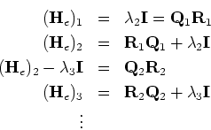
Perform QR factorization:
Obtain New Iterate:
Then
![]() is similar to
is similar to
![]() because
because
![\begin{eqnarray*}({\bf He})_{k+1} & = & {\bf Q}^T_k{\bf Q}_k {\bf R}_k
{\bf Q}_...
...I] {\bf Q}_k\\
\\
& = & {\bf Q}_k^T ({\bf H}_e)_k {\bf Q}_k .
\end{eqnarray*}](img40.gif)
For double or complex eigenvalues
the shift strategy has to change in order to deal effectively
with the ``bumps'' in the diagonal of the ![]() matrix,
as discussed earlier. Specifically, we modify the algorithm so that
each iteration has two substeps. We can use the eigenvalues
matrix,
as discussed earlier. Specifically, we modify the algorithm so that
each iteration has two substeps. We can use the eigenvalues
![]() and
and ![]() of the submatrix
to obtain the iterates as follows
of the submatrix
to obtain the iterates as follows

Remark: After the last eigenvalue ![]() has been obtained, deflation of the Hessenberg matrix
can be applied to find the next one at
reduced computational cost. In general, it takes about
two to three QR iterations to compute one eigenvalue.
The total cost is about
has been obtained, deflation of the Hessenberg matrix
can be applied to find the next one at
reduced computational cost. In general, it takes about
two to three QR iterations to compute one eigenvalue.
The total cost is about
![]() but such an
operation count is approximate and problem dependent.
but such an
operation count is approximate and problem dependent.
The Symmetric QR Eigensolver: Wilkinson Shift
Symmetric matrices are special, first because they have
only real eigenvalues but also because the
Hessenberg transformation reduces the matrix to a symmetric
tridiagonal matrix. The QR iteration maintains
this property for the entire sequence. The other good news is that the
QR factorization of a symmetric tridiagonal matrix costs
only
![]() ,
instead of
,
instead of
![]() for the Hessenberg matrix.
Therefore, the computational cost in this case is
for the Hessenberg matrix.
Therefore, the computational cost in this case is
![]() times the number of iterations to converge to all eigenvalues.
times the number of iterations to converge to all eigenvalues.
Wilkinson[#!Wilkinson!#] has suggested that instead
of using the
h(k)nn as the shift ![]() to accelerate convergence, a more effective way
is to use the eigenvalue of the
to accelerate convergence, a more effective way
is to use the eigenvalue of the ![]() matrix
matrix
![\begin{displaymath}\left [ \begin{array}{cc}
h_{n-1,n-1} & h_{n,n-1}\\
h_{n,n-1} & h_{nn}\end{array}\right ]\end{displaymath}](img45.gif)
Parallel QR Eigensolver: Divide-and-Conquer
A fully parallel algorithm for the symmetric eigenvalue problem was developed by Dongara and Sorensen [#!DogaraS87!#]. It is based on the QR iteration and the divide-and-conquer approach we have encountered many times in this book.
First, we tridiagonalize the full symmetric matrix
![]() ,
where the latter has the form
,
where the latter has the form
![\begin{displaymath}{\bf T} = \left [ \begin{array}{cccccc}
a_1 & b_1 \\
b_1 & a...
...hspace*{-.3in}b_{n-1} & \hspace*{-.3in}a_n
\end{array}\right ]\end{displaymath}](img48.gif)
![\begin{displaymath}{\bf T}_1 = \left [ \begin{array}{ccccccccc}
a_1 & b_1\\
b_1...
... & \hspace*{-.3in}a_k & \hspace*{-.3in}-b_k
\end{array}\right ]\end{displaymath}](img50.gif)
![\begin{displaymath}{\bf T}_2 = \left [ \begin{array}{ccccccccccccc}
a_{k+1}-b_k ...
...& b_{n-1}\\
&\hspace*{.5in} b_{n-1} && a_n \end{array}\right ]\end{displaymath}](img51.gif)
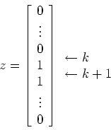
![\begin{displaymath}{\bf T} = \left [ \begin{array}{cc}
{\bf T}_1 & 0\\
0 & {\bf T}_2\end{array}\right ] + b_k {\bf z}\end{displaymath}](img52.gif)

![\begin{displaymath}{\bf D}_1 =\left [ \begin{array}{ccccccccccc}
d_1\\
& d_2 & ...
...{\large0}\\
{\large0} && \ddots \\
&&& d_n\end{array}\right ]\end{displaymath}](img59.gif)
![\begin{displaymath}\mbox{\boldmath $\xi$ }= \left [ \begin{array}{cc}
{\bf Q}_1 & 0\\
0 & {\bf Q}_2 \end{array} \right ]^T {\bf z}\end{displaymath}](img60.gif)
![\begin{displaymath}{\bf T} = \left [ \begin{array}{cc}
{\bf Q}_1 & 0 \\
0 & {\b...
...eft [ \begin{array}{cc}
Q_1 & 0\\
0 & Q_L\end{array}\right ]^T\end{displaymath}](img61.gif)

![\begin{displaymath}{\bf v}_i = \left [ \begin{array}{cc}
{\bf Q}_1 & 0\\
0 & {\bf Q}_2 \end{array}\right ] {\bf y}_i.
\end{displaymath}](img69.gif)
Reference: J. Dongarra and D.C. Sorensen, ``A fully parallel algorithm for the symmetric eigenvalue problem'', SIAM J. Sci. and Stat. Comp., vol. 8, p. S139-S154, (1987).