next up previous
Next: About this document ...

Eigenvalues and Eigenvectors


The eigenvalues and corresponding eigenvectors of a matrix ${\bf A}$ are determined by solving

\begin{displaymath}{\bf A}{\bf x} = \lambda {\bf x} \Rightarrow
({\bf A} -\lambda {\bf I}){\bf x}=0\end{displaymath}

where

\begin{displaymath}{\bf I} = \left [ \begin{array}{cccccccc}
\par 1 & & \\
& 1 ...
...ge0} \\
{\Large0} & & & \ddots\\
& & & & 1
\end{array}\right]\end{displaymath}

is the identity matrix. The eigenvectors ${\bf x}$ are non-zero if the determinant is zero, i.e.,

\begin{displaymath}\det (A-\lambda I) =0,
\end{displaymath}

and this equation determines the eigenvalues $\lambda$. It can be re-written as

\begin{displaymath}\det (A-\lambda I)= \Pi^n_{i=1} (a_{ii}-\lambda_i) + p_{n-1}(\lambda) = 0,
\end{displaymath}

where aii are the diagonal elements of ${\bf A}$ and $p_{n-1}(\lambda)$ is a (n-1)th-order polynomial. Therefore, an $n\times n$ matrix has exactly n eigenvalues, i.e. the roots of the above nth-order polynomial, which may be real or complex and simple or multiple. However, the above approach is rarely used in practice to compute the eigenvalues because it is computationally very expensive and also unstable. This is illustrated with the Wilkinson matrix

\begin{displaymath}W= \left [ \begin{array}{ccccccccccc}
1\\
&2 & \\
& & 3 & &...
... & & & \ddots\\
& & & & 19\\
& & & & & 20
\end{array}\right ]\end{displaymath}

where by ${\cal O}(\epsilon)$ we denote possible round-off error. In the absence of round-off the eigenvalues are determined by

\begin{displaymath}(1-\lambda) (2-\lambda)(3-\lambda) \ldots (19-\lambda) (20-\lambda) = 0,
\end{displaymath}

and thus: $\lambda_i = i.$ However, for $\epsilon \not= 0$ the characteristic polynomial is

\begin{displaymath}\lambda^{20}-210 \lambda^{19} + \ldots + 20! + \epsilon \lambda^{19}.\end{displaymath}

Let us assume that $\epsilon = 10^{-11}$ (i.e., slightly below the double-precision machine accuracy), then we obtain

\begin{displaymath}\lambda_i = 1, 2, \ldots, 8,9, 10.01, 11.3, 12.5 \pm 0.5i, 14.5 \pm 0.5 i, \ldots, 20.\end{displaymath}

Therefore, the presence of even slight noise in the data results in several eigenvalues being wrong, even complex in this case!


Next, we provide some basic background on linear algebra. First, we define the similarity transformation. Specifically, we say that the matrix ${\bf A}$ is similar to matrix ${\bf B}$ if ${\bf A}$ and ${\bf B}$ have the same eigenvalues (i.e. the same eigenspectrum) but not necessarily the same eigenvectors. Therefore, the transformation

\begin{displaymath}{\bf A} \longrightarrow {\bf P}{\bf A}{\bf P}^{-1}\end{displaymath}

where ${\bf P}$ is a non-singular matrix, leads to a matrix ${\bf B} = {\bf P} A {\bf P}^{-1}$ which is similar to ${\bf A}$. This can be proved based on the definitions. Let us assume

\begin{displaymath}{\bf A}{\bf x} = \mbox{\boldmath $\lambda$} {\bf x}\end{displaymath}

and

\begin{displaymath}{\bf P} {\bf A}{\bf P}^{-1} y = \mbox{\boldmath $\mu$} {\bf y}.\end{displaymath}

Then

\begin{displaymath}{\bf A}{\bf P}^{-1}{\bf y} = {\bf P}^{-1} \mu {\bf y} =
\mu {\bf P}^{-1}{\bf y}
\end{displaymath}

and by defining ${\bf x}={\bf P}^{-1} {\bf y}$, we have $\mu =\lambda$, so all n eigenvalues are the same for both ${\bf A}$ and ${\bf P}{\bf A}{\bf P}^{-1}.$ We also note that if ${\bf P}$ is an orthogonal matrix then ${\bf P}^{-1} = P^{T}$ and then ${\bf P}{\bf A}{\bf P}^T$ is similar to ${\bf A}.$ In theory, any non-singular matrix ${\bf P}$can be used in the similarity transformation but the best choice in practice is to use an orthonormal matrix. The reason is that with finite arithmetic ill-conditioned amplify the round-off error and may lead to erroneous results unlike orthonormal matrices.


Remark 1: The transpose matrix ${\bf A}^T$ is similar to matrix ${\bf A}$ since they have the same characteristic polynomial. However, they do not have the same eigenvectors. In contrast, the inverse matrix ${\bf A}^{-1}$ has the same eigenvectors with ${\bf A}$ but inverse eigenvalues, $\lambda^{-1}_i$. This is true because

\begin{displaymath}{\bf A} {\bf x} = \lambda {\bf x} \Rightarrow {\bf x} =
{\bf...
...bda {\bf x} \Rightarrow \lambda^{-1} {\bf x} = A^{-1} {\bf x}.
\end{displaymath}


Remark 2: The matrix ${\bf A}^{k}$, where k is a positive integer has eigenvalues $\lambda^k$, where $\lambda$ are the eigenvalues of ${\bf A}$. However, ${\bf A}^{k}$ and ${\bf A}$ have the same eigenvectors. This can be extended further and it is easy to show that if we construct a polynomial matrix:

\begin{displaymath}p({\bf A}) \equiv \alpha_0 {\bf A}^0 +
\alpha_1 {\bf A} + \alpha_2 A^2 + \ldots + \alpha_k{\bf A}^k
\end{displaymath}

then

\begin{displaymath}p(\lambda_1), \, p(\lambda_2), \, p(\lambda_3) \, \ldots \, p(\lambda_n)
\end{displaymath}

are the eigenvalues of $p({\bf A})$. Also, the eigenvectors of ${\bf A}$ are also eigenvectors of $p({\bf A})$. As an example, the eigenvalues of $p_1({\bf A}) = {\bf A} + \sigma {\bf I}$ are $(\lambda_i + \sigma).$


We have already seen that computing the eigenvalues accurately from the determinant may not always be possible, although the Newton-Raphson method of chapter [*] is an accurate method of computing the roots of polynomials but it may be inefficient. In the following, we present a simple method to compute iteratively and selectively the maximum and minimum eigenvalues and corresponding eigenvectors.


Power Method


This is a very simple method to obtain the maximum eigenvalue. The main idea is to obtain iterates from

\begin{displaymath}{\bf x}^{k+1} = c{\bf A}x^k,
\end{displaymath}

where c is a normalization constant that prevents ${\bf x}^{k+1}$ from becoming too large. After many iterations $(k\rightarrow \infty)$, xk+1 will converge to the eigenvector ${\bf v} _1$ of ${\bf A}$ corresponding to the maximum eigenvalue $\lambda_1$. Here, we assume that there exists an eigenvalue $\lambda_1$ which dominates, i.e.,

\begin{displaymath}\lambda_1 > \lambda_2 \geq \lambda_3 \ldots \geq \lambda_n.\end{displaymath}

We can initialize this iteration by an arbitrary (non-zero) vector ${\bf x}^0.$

To see why this process converges and at what rate we project the initial guess ${\bf x}^0$ to the space spanned by all the eigenvector ${\bf v}_i$ of ${\bf A}$, i.e.,

\begin{displaymath}{\bf x}^0 = c_1 {\bf v}_1 +c_2 {\bf v}_2 \ldots + \ldots + c_n {\bf v}_n\end{displaymath}

and thus

\begin{displaymath}{\bf x}^k = {\bf A}{\bf x}^{k-1} = \ldots = A^k {\bf x}^0 =
c_1 \lambda^k_1 {\bf v}_1 + \ldots + c_n\lambda^k_n{\bf v}_n
\end{displaymath}

then, we see that

\begin{displaymath}\frac{{\bf x}^k}{c_1 \lambda^k_1} = {\bf v}_1 +
\frac{c_2}{c...
...}{c_1} \left ( \frac{\lambda_n}{\lambda_1}\right )^k
{\bf v}_n\end{displaymath}

converges to ${\bf v} _1$ because all factors

\begin{displaymath}\left (\frac{\lambda_i}{\lambda_1}\right )^k, \, i \not= 1\end{displaymath}

are less than one and tend to zero for $k\rightarrow \infty.$

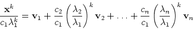
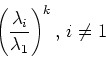
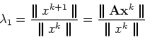
The convergence rate is determined by the relative convergence of the second largest to the largest term, i.e., the ratio

\begin{displaymath}\frac{\vert\lambda_2\vert}{\vert\lambda_1\vert},\end{displaymath}

which represents the most resistive contribution to the error. The smaller this ratio is the faster the convergence is!

A pseudo-code for this algorithm is:
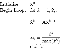

\begin{displaymath}\begin{array}{ll}
\mbox{Initialize} & {\bf x}^0\\
\mbox{{\rm...
...c{\hat{x}^k}{\max (\hat{x}^k)}}\\
& \mbox{end for}
\end{array}\end{displaymath}

Upon termination of the loop, $\max (\hat{x}^k) \rightarrow \lambda_1$ and ${\bf x}^k \rightarrow {\bf v}_1$. Note that here $\max(\hat{x}^k)$ denotes the maximum entry in the vector ${\bf x}^k$, and is simply used for normalization.


In the algorithm above the value of $\lambda_1$ is estimated from the maximum component of ${\bf x}^k.$ However, any other norm can be used, e.g., the L2 norm
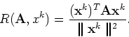
\begin{displaymath}\lambda_1 = \frac{\parallel x^{k+1}\parallel}{\parallel x^k\p...
...ac{\parallel {\bf A}{\bf x}^k\parallel}{\parallel x^k\parallel}\end{displaymath}

or alternatively the eigenvalue can be computed via the Rayleigh quotient. This is defined by

\begin{displaymath}R({\bf A}, x^k) =
\frac{({\bf x}^k)^T{\bf A}{\bf x}^k}{\parallel {\bf x}^k\parallel^2}.
\end{displaymath}

If ${\bf x} = {\bf v}_1$, i.e., the first eigenvector, then obviously $R({\bf A}, {\bf v}_1) = \lambda_1.$ In general, if ${\bf A}$ is a symmetric matrix and ${\bf x}$ is a close approximation to the eigenvector ${\bf v} _1$ the Rayleigh quotient is close to the corresponding eigenvalue $\lambda_1.$ This can be seen by projecting ${\bf x } = \sum^n_{i=1} c_i {\bf v}_i$, as before, where ${\bf v}_i$ are orthonormal due to symmetry of ${\bf A}$, and ${\bf v}_i^T {\bf v}_i = 1.$ Then

\begin{eqnarray*}R({\bf A}, x) & = & \frac{{\bf x}^T {\bf A}{\bf x}}{{\bf x}^T{\...
...right )^2 +
\ldots + \left (\frac{c_n}{c_1}\right )^2}\right ].
\end{eqnarray*}


However, due to our assumption that ${\bf x} \approx {\bf v}_1
\Rightarrow c_1 \gg c_i$, $\forall i \not=1.$ Thus, the quantity in brackets tends to 1 and so $R({\bf A},{\bf x})$ tends to $\lambda_1.$

The convergence of the power method can be enhanced by shifting the eigenvalues, so instead of multiplying the initial guess by powers of ${\bf A}$we multiply by powers of $(A - \sigma I)$ which has eigenvalues $(\lambda_i - \sigma)$ while the eigenvectors remain the same. The corresponding convergence rate is then estimated by

\begin{displaymath}\left \vert \frac{\lambda_2 - \sigma}{\lambda_1 - \sigma}\right \vert.
\end{displaymath}

If all the eigenvalues are real, the best shift is either

\begin{displaymath}\sigma = \frac{1}{2} (\lambda_2 + \lambda_n)\;\; {\rm or} \;\;
\sigma = \frac{1}{2} (\lambda_1+ \lambda_{n-1})\end{displaymath}

if $(\lambda_1 - \lambda_2)$ or $(\lambda_{n-1} -
\lambda_n)$ is larger, respectively.


The Inverse Shifted Power Method


In order to compute selectively the smallest eigenvalue we can apply again the power method by multiplying by powers of the inverse, i.e., ${\bf A}^{-1}.$ Thus, the iteration procedure here is

\begin{displaymath}{\bf A}{\bf x}^{k+1} = c {\bf x}^k,
\end{displaymath}

where again c is a normalization constant. This method is most effective with a proper shift, so the modified iteration is

\begin{displaymath}({\bf A} - \sigma I){\bf x}^{k+1} = {\bf x}^k\end{displaymath}

and the solution will converge to the smallest shifted eigenvalue $\vert\lambda_n-\sigma\vert$ and the corresponding eigenvector, assuming that the shift $\sigma$ is close to $\lambda_n$ (the smallest eigenvalue). The rate of convergence is now

\begin{displaymath}\frac{\vert\lambda_n-\sigma \vert}{\vert\lambda_{n-1}-\sigma \vert}\end{displaymath}

so if $\sigma$ is close to $\lambda_n$, the above ratio is very small and convergence is very fast. Clearly, if $\sigma$ is close to any other eigenvalue $\lambda_i$the the corresponding contribution dominates and then we obtain the eigenpair $(\lambda_i, {\bf v}_i$.

The following pseudo-code summarizes the algorithm:


\begin{displaymath}\begin{array}{llll}
\mbox{Initialize:} & \mbox{Choose}\; {\bf...
...
& \mbox{{\rm else if continue}}\\
& \mbox{Endfor}
\end{array}\end{displaymath}

Upon termination, ${\bf x}^k$ converges to the desired eigenvector and the corresponding eigenvalue can be computed from the Rayleigh quotient.


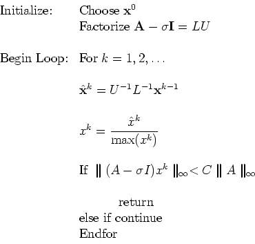
Remark 1: Note that we do not actually compute explicitly the inverse ${\bf A}^{-1}$ or $({\bf A}-\sigma {\bf I})^{-1}$ but we simply do an LU factorization only once outside the loop. So the computational complexity of this algorithm is ${\cal O}(n^2)$ times the number of iterations plus the initial ${\cal O}(2n^3/)$ cost for the LU factorization.


Remark 2: To accelerate convergence, we can start with a few iterations using the standard power method, obtain a first good guess and corresponding shift $\sigma$ via the Rayleigh quotient, and then switch to the inverse iteration method.


Remark 3: The matrix $({\bf A} -\sigma {\bf I})$ is ill-conditioned, however in practice the error associated with this seems to favor the inverse iteration as it grows toward the direction of the desired eigenvector. Therefore, the inverse shifted power method is a stable method.


We can modify the inverse shifted power method and enhance convergence even more (to third-order) if we update the value of the shift adaptively using the Rayleigh quotient. The following algorithm presents this modification :


\begin{displaymath}\begin{array}{lllll}
\mbox{Initialize:} & \mbox{Choose}\; {\b...
...{{\rm else if continue}}\\
& \mbox{{\rm End Loop}}
\end{array}\end{displaymath}


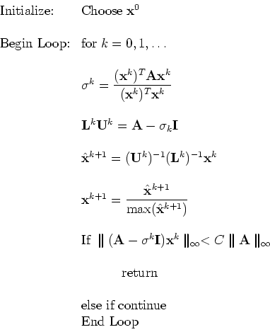
Remark: While this algorithm triples the number of correct digits in each iteration it requires ${\cal O}(n^3)$ work at each iteration because the matrix $({\bf A} - \sigma_k{\bf I})$ changes in each iteration. A more economical approach is to ``freeze'' $\sigma_k$ for a few iterations so that the LU decomposition is not employed in each iteration. The resulted convergence rate is then less than cubic but overall this is a more efficient approach.


next up previous
Next: About this document ...
George Karniadakis
2001-11-01