The Lanczos Eigensolver

This algorithm, developed by Lanczos in the 1950s, is particularly useful for large symmetric matrices, which are sparse. The QR method can also be used for such systems but it does not maintain the sparsity of the new matrices in each iteration and thus it becomes inefficient.

The key idea in Lanczos's approach is to make use of all the previous iterates

$${\bf v}, {\bf A}, {\bf v}, {\bf A}^2 {\bf v}, \ldots {\bf A}^{k-1} {\bf v}$$

produced in a power method iteration. These k vectors form the so-called Krylov space:

$${\cal K}_k({\bf A}_1 {\bf v}) = \; {\rm span}\; \{ {\bf v}, {\bf A}{\bf v}, {\bf A}^2 {\bf v} \ldots, A^{k-1}\}$$

of dimension k. In principle, after n iterations assuming that all

$${\bf v}, {\bf A}{\bf v}, \ldots, {\bf A}^{n-1}{\bf v}$$

are linearly independent, we can express any vector ${\bf x}$ in terms of the basis formed by the vectors generated by that sequence. However, this sequence is not computationally friendly and there is a bias towards the maximum (or minimum) eigenvalues of ${\bf A}.$ The idea is then to orthogolanize these vectors but do it fast, that is don't use Gram-Schmidt or QR but something new!. The new orthonormalization will be based on the magic 3-term recurrence formula! We have already seen how to do that in the context of orthogonal polynomials (see section ) and also in the conjugate gradient method (see ).

Assuming that we have produced the orthonormal vectors

$${\bf q}_1, \, {\bf q}_2, \, \ldots, \, {\bf q}_k$$

then we can construct the orthornormal matrix ${\bf Q}$ by employing bf q_i as its columns, and we have that

$${\bf Q}^T{\bf Q} = {\bf I},$$

that is the condition of orthonormality.

We can then transform ${\bf A}$ to its similar matrix ${\bf T}$ suing the similarity transformation, ie.

$${\bf Q}^T {\bf A}{\bf Q} = {\bf T}\; {\rm or}\; {\bf A}{\bf Q} = {\bf Q} {\bf T}$$

where ${\bf T}$ is a tridiagonal matrix of the form

$$T_k = \left [ \begin{array}{ccccccccccccc} & & \alpha_1 && \... ... &&& \beta_{ky} & &\alpha_k & &\beta_{k-1}\end{array}\right ].$$

The tridigonal structure of T is due to the 3-term magic formula so the columns of ${\bf Q}$ satisfy

$${\bf A} {\bf q}_i = \beta_{i-1} {\bf q}_{i-1} + \alpha_i {\bf q}_i + \beta_i {\bf q}_{i+1}\;\; i=1,2,\ldots$$

We can compute now the coefficients $\alpha_i$ and $\beta_i$ from the orthonormality conditions. First multiplying the above equation by ${\bf q}^T_i$ we obtain

$${\bf q}_i^T {\bf A}{\bf q}_i = \beta_{i-1}{\bf q}^T_i {\bf q}... ... _i {\bf q}_i^T {\bf q}_i + \beta_i {\bf q}^T_i {\bf q}_{i+1},$$

where ${\bf q}_i^T {\bf q}_i =1$, and also ${\bf q}_i^T {\bf q}_{i-1} = 0; {\bf q}^T_i {\bf q}_{i+1} = 0$ due to orthonormality condition. Therefore, from this equation we obtain

$$\alpha_i = {\bf q}_i^T {\bf A}{\bf q}_i.$$

Conversely, assuming that $\alpha_i$ is obtained from the above formula we can prove that ${\bf q}_{i+1} \perp {\bf q}_i$ by induction.

The coefficient $\beta_i$ is also obtained from the recurrence formula

$${\bf r}_i \equiv \beta_i {\bf q}_{i+1} = {\bf A} {\bf q}_i - \alpha_i {\bf q}_i - \beta_{i-1} {\bf q}_{i-1}$$

if we further assume that

$$\beta_i \not= 0 \Rightarrow \beta_i = \parallel {\bf r}_i \parallel_2$$

and

$${\bf q}_{i+1} = \frac{{\bf r}_i}{\beta_i}.$$

All vector ${\bf q}_{i+1}$ generated by the 3-term sequence are orthogonal to all ${\bf q}_k$, k< i given the symmetry of the matrix ${\bf A}$. This can be proved by induction. First, we assume that

$${\bf q}_{i+1} \perp {\bf q}_{i}\; {\rm and}\; {\bf q}_{i+1} \perp {\bf q}_{i-1}$$

and also that from the previous step (of the induction process) we have already that the condition

$${\bf q}_i \perp {\bf q}_k, \quad k < i$$

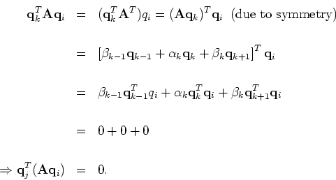
is valid. We will then prove that ${\bf q}_{i+1} \perp {\bf q}_k$but first we prove that the vectors ${\bf q}_k$ and ${\bf q}_i$ are A-orthogonal. For this, we multiply the 3-term recurrence formula by ${\bf q}_k$ $(k\leq i-2)$

$$\begin{eqnarray*}{\bf q}_k^T {\bf A}{\bf q}_i & = & ({\bf q}^T_k {\bf A}^T)q_i =... ... + 0\\ \\ \Rightarrow {\bf q}^T_j({\bf A} {\bf q} _i)& = & 0. \end{eqnarray*}$$

Now, multiplying the 3-term formula again we have

$$\beta_i {\bf q}^T_k q_{i+1} = {\bf q}^T_k{\bf A} q_i - \alph... ...bf q}^T_k q_i - \beta_i {\bf q}^T_k {\bf q}_{i-1} = 0 + 0 + 0,$$

so we have proved by induction that ${\bf q}_{i+1}$ is orthogonal to all previous ${\bf q}_i$. We note here that each induction step has two substeps, as presented above, first to show the A-orthogonality and then the final result.

In practice, the problem is that the orthogonality is not preserved. In fact, as soon as one eigenvalue converges all the basis vectors ${\bf q}_i$ pick up perturbations biased toward the direction of the corresponding eigenvector and orthogonality is lost. This has been analyzed in detail by Paige [#!Paige!#] who found that a ``ghost'' copy of the eigenvalue will appear again in the tridiagonal matrix ${\bf T}.$ The straightforward remedy is to fully re-orhonormalize the sequence by using Gram-Schmidt or even QR. However, either approach would be expense if the dimension if the Krylov space is large, so instead a selective re-orthonormalization is pursued. More specifically, the practical approach is to orthonormalize half-way i.e., within half machine-recision $\sqrt{\epsilon_M}$ [#!Templates2!#].

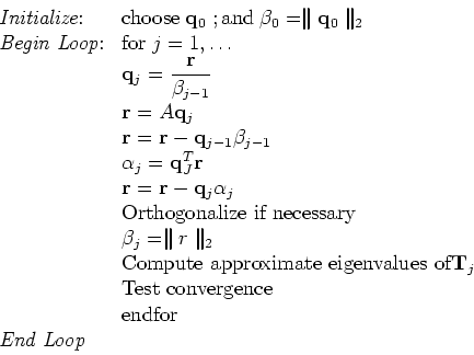
The following algorithm presents an orthogonalized version of the basic Lanczos algorithm for symmetric matrices.

$$\begin{array}{lll} \mbox{{\em Initialize}:} & \mbox{choose}\;... ...ence}}\\ & \mbox{endfor}\\ \mbox{{\em End Loop}} \end{array}$$

Remark 1: If the eigenvalues of ${\bf A}$ are not well separated, then we can use a shift and employ the matrix

$$({\bf A} - \sigma {\bf I})^{-1}$$

following the shifted inverted power method to generate the appropriate Krylov subspaces.

Remark 2: The Lanczos algorithm can be extended to non-symmetric systems - see references in [#!Saad!#], [#!Templates!#].