Here are some examples of calculus symbolic computations using Sage. They use the Maxima interface.
Work is being done to make the commands for the symbolic calculations given below more intuitive and natural. At the moment, we use the maxima class interface.
Sage knows how to differentiate and integrate many functions. For example, to
differentiate \( \sin (u) \) with respect to u, do the following:
sage: u = var('u')
sage: diff(sin(u), u)
cos(u)
Differentiation:
sage: var('x k w')
(x, k, w)
sage: f = x^3 * e^(k*x) * sin(w*x); f
x^3*e^(k*x)*sin(w*x)
sage: f.diff(x)
w*x^3*cos(w*x)*e^(k*x) + k*x^3*e^(k*x)*sin(w*x) + 3*x^2*e^(k*x)*sin(w*x)
sage: latex(f.diff(x))
w x^{3} \cos\left(w x\right) e^{\left(k x\right)} + k x^{3} e^{\left(k x\right)} \sin\left(w x\right) + 3 \, x^{2} e^{\left(k x\right)} \sin\left(w x\right)
If you type view(f.diff(x)) another window will open up displaying the compiled output. In the notebook, you can enter
var('x k w')
f = x^3 * e^(k*x) * sin(w*x)
show(f)
show(f.diff(x))
into a cell and press shift-enter for a similar result. You can also differentiate and integrate using the commands
R = PolynomialRing(QQ,"x")
x = R.gen()
p = x^2 + 1
show(p.derivative())
show(p.integral())
in a notebook cell, or
sage: R = PolynomialRing(QQ,"x")
sage: x = R.gen()
sage: p = x^2 + 1
sage: p.derivative()
2*x
sage: p.integral()
1/3*x^3 + x
on the command line. At this point you can also type view(p.derivative()) or view(p.integral()) to open a new window with output typeset by LaTeX.
You can find critical points of a piecewise defined function:
sage: x = PolynomialRing(RationalField(), 'x').gen()
sage: f1 = x^0
sage: f2 = 1-x
sage: f3 = 2*x
sage: f4 = 10*x-x^2
sage: f = Piecewise([[(0,1),f1],[(1,2),f2],[(2,3),f3],[(3,10),f4]])
sage: f.critical_points()
[5.0]
Taylor series:
sage: var('f0 k x')
(f0, k, x)
sage: g = f0/sinh(k*x)^4
sage: g.taylor(x, 0, 3)
-62/945*f0*k^2*x^2 + 11/45*f0 - 2/3*f0/(k^2*x^2) + f0/(k^4*x^4)
sage: maxima(g).powerseries('_SAGE_VAR_x',0)    # TODO: write this without maxima
16*_SAGE_VAR_f0*('sum((2^(2*i1-1)-1)*bern(2*i1)*_SAGE_VAR_k^(2*i1-1)*_SAGE_VAR_x^(2*i1-1)/factorial(2*i1),i1,0,inf))^4
Of course, you can view the LaTeX-ed version of this using view(g.powerseries('x',0)).
The Maclaurin and power series of \(\log({\frac{\sin(x)}{x}})\):
sage: f = log(sin(x)/x)
sage: f.taylor(x, 0, 10)
-1/467775*x^10 - 1/37800*x^8 - 1/2835*x^6 - 1/180*x^4 - 1/6*x^2
sage: [bernoulli(2*i) for i in range(1,7)]
[1/6, -1/30, 1/42, -1/30, 5/66, -691/2730]
sage: maxima(f).powerseries(x,0)    # TODO: write this without maxima
'sum((-1)^i3*2^(2*i3-1)*bern(2*i3)*_SAGE_VAR_x^(2*i3)/(i3*factorial(2*i3)),i3,1,inf)
Numerical integration is discussed in Riemann and trapezoid sums for integrals below.
Sage can integrate some simple functions on its own:
sage: f = x^3
sage: f.integral(x)
1/4*x^4
sage: integral(x^3,x)
1/4*x^4
sage: f = x*sin(x^2)
sage: integral(f,x)
-1/2*cos(x^2)
Sage can also compute symbolic definite integrals involving limits.
sage: var('x, k, w')
(x, k, w)
sage: f = x^3 * e^(k*x) * sin(w*x)
sage: f.integrate(x)
((24*k^3*w - 24*k*w^3 - (k^6*w + 3*k^4*w^3 + 3*k^2*w^5 + w^7)*x^3 + 6*(k^5*w + 2*k^3*w^3 + k*w^5)*x^2 - 6*(3*k^4*w + 2*k^2*w^3 - w^5)*x)*cos(w*x)*e^(k*x) - (6*k^4 - 36*k^2*w^2 + 6*w^4 - (k^7 + 3*k^5*w^2 + 3*k^3*w^4 + k*w^6)*x^3 + 3*(k^6 + k^4*w^2 - k^2*w^4 - w^6)*x^2 - 6*(k^5 - 2*k^3*w^2 - 3*k*w^4)*x)*e^(k*x)*sin(w*x))/(k^8 + 4*k^6*w^2 + 6*k^4*w^4 + 4*k^2*w^6 + w^8)
sage: integrate(1/x^2, x, 1, infinity)
1
You can find the convolution of any piecewise defined function with another (off the domain of definition, they are assumed to be zero). Here is \(f\), \(f*f\), and \(f*f*f\), where \(f(x)=1\), \(0<x<1\):
sage: x = PolynomialRing(QQ, 'x').gen()
sage: f = Piecewise([[(0,1),1*x^0]])
sage: g = f.convolution(f)
sage: h = f.convolution(g)
sage: P = f.plot(); Q = g.plot(rgbcolor=(1,1,0)); R = h.plot(rgbcolor=(0,1,1))
To view this, type show(P+Q+R).
Regarding numerical approximation of \(\int_a^bf(x)\, dx\), where \(f\) is a piecewise defined function, can
sage: f1(x) = x^2
sage: f2(x) = 5-x^2
sage: f = Piecewise([[(0,1),f1],[(1,2),f2]])
sage: f.trapezoid(4)
Piecewise defined function with 4 parts, [[(0, 1/2), 1/2*x],
[(1/2, 1), 9/2*x - 2], [(1, 3/2), 1/2*x + 2],
[(3/2, 2), -7/2*x + 8]]
sage: f.riemann_sum_integral_approximation(6,mode="right")
19/6
sage: f.integral()
Piecewise defined function with 2 parts,
[[(0, 1), x |--> 1/3*x^3], [(1, 2), x |--> -1/3*x^3 + 5*x - 13/3]]
sage: f.integral(definite=True)
3
Numerical integration methods can prove useful if the integrand is known only at certain points or the antiderivate is very difficult or even impossible to find. In education, calculating numerical methods by hand may be useful in some cases, but computer programs are usually better suited in finding patterns and comparing different methods. In the next example, three numerical integration methods are implemented in Sage: the midpoint rule, the trapezoidal rule and Simpson's rule. The differences between the exact value of integration and the approximation are tabulated by the number of subintervals n
sage: f(x) = x^2-3
sage: a = 0.0
sage: b = 2.0
sage: table = []
sage: exact = integrate(f(x), x, a, b)
sage: for n in [4, 10, 20, 50, 100]:
....:     h = (b-a)/n
....:     midpoint = sum([f(a+(i+1/2)*h)*h for i in range(n)])
....:     trapezoid = h/2*(f(a) + 2*sum([f(a+i*h) for i in range(1,n)])
....:     + f(b))
....:     simpson = h/3*(f(a) + sum([4*f(a+i*h) for i in range(1,n,2)])
....:     + sum([2*f(a+i*h) for i in range (2,n,2)]) + f(b))
....:     table.append([n, h.n(digits=2), (midpoint-exact).n(digits=6),
....:     (trapezoid-exact).n(digits=6), (simpson-exact).n(digits=6)])
....:     html.table(table, header=["n", "h", "Midpoint rule",
....:     "Trapezoidal rule", "Simpson's rule"])
There are also built-in methods for numerical integration in Sage.
For instance, it is possible to automatically produce piecewise-defined
line functions defined by the trapezoidal rule or the midpoint rule.
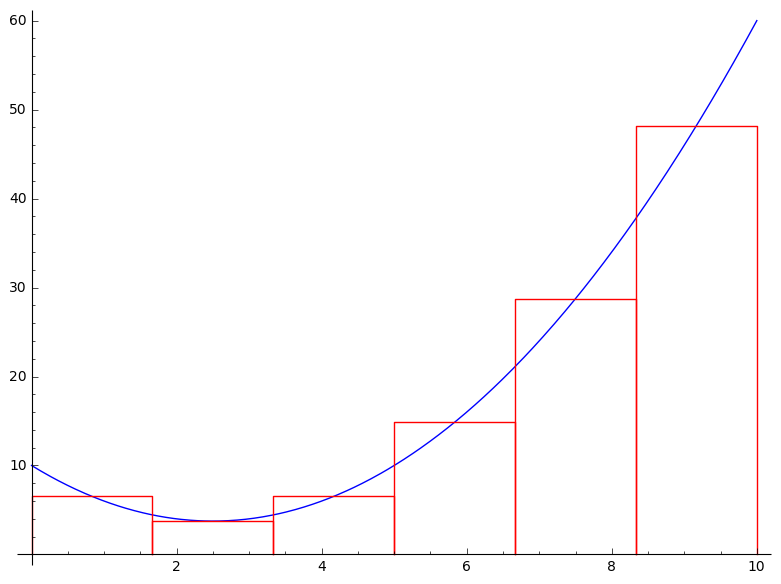
These functions can be used to visualize different geometric interpretations of the numerical integration methods. In the next example,
midpoint rule is used to calculate an approximation for the definite
integral of the function
f(x) =x^2 -5x + 10
over the interval [0;10] using six subintervals
sage: f(x) = x^2-5*x+10
sage: f = Piecewise([[(0,10), f]])
sage: g = f.riemann_sum(6, mode="midpoint")
sage: F = f.plot(color="blue")
sage: R = add([line([[a,0],[a,f(x=a)],[b,f(x=b)],[b,0]], color="red") for (a,b), f in g.list()]
sage: show(F+R)
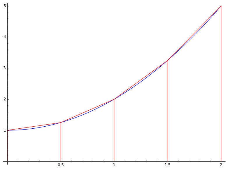
The Trapezoid Rule approximates the area under a given curve by finding the area under a linear approximation to the curve. The linear segments are given by the secant lines through the endpoints of the subintervals: for f(x)=x^2+1 on [0,2] with 4 subintervals, this looks like:
sage: x = var('x')
sage: f1(x) = x^2 + 1
sage: f = Piecewise([[(0,2),f1]])
sage: trapezoid_sum = f.trapezoid(4)
sage: P = f.plot(rgbcolor=(0,0,1), plot_points=40)
sage: Q = trapezoid_sum.plot(rgbcolor=(1,0,0), plot_points=40)
sage: L = add([line([[a,0],[a,f(x=a)]], rgbcolor=(1,0,0)) for (a,b), f in trapezoid_sum.list()])
sage: M = line([[2,0],[2,f1(2)]], rgbcolor=(1,0,0))
sage: show(P + Q + L + M)
To integrate the function cos(2*x)^4 +sin(x) we do
sage: numerical_integral(lambda x: cos(2*x)^5 + sin(x),  0, 2*pi)
(2.3561944901923457, 5.322071926740605e-14)
The input can be any callable:
sage: numerical_integral(lambda x: cos(2*x)^5 + sin(x),  0, 2*pi)
(2.3561944901923457, 5.322071926740605e-14)
We check this with a symbolic integration:
sage: (cos(2*x)^4+sin(x)).integral(x,0,2*pi)
3/4*pi
It is possible to integrate on infinite intervals as well by using +Infinity or -Infinity in the interval argument. For example:
sage: f = exp(-2*x)
sage: numerical_integral(f, 0, +Infinity)
(0.4999999999993456, 2.5048509541974486e-07)
We can also numerically integrate symbolic expressions using either this function (which uses GSL) or the native integration (which uses Maxima):
sage: (x^3*sin(1/x)).nintegral(x,0,pi)
(9.874626194990983, 6.585622218041451e-08, 315, 0)
Computing the solution of some given equation is one of the fundamental problems of numerical analysis. If a real-valued function is differentiable and the derivative is known, then Newton's method may be used to find an approximation to its roots. In Newton's method, an initial guess \( x_0 \) for a root of the differentiable function \( f: \,\mathbb{R} \mapsto \mathbb{R} \) is made. The consecutive iterative steps are defined by
The function
newton_method is used
to generate a list of the iteration points. Sage contains a preparser
that makes it possible to use certain mathematical constructs such as
\( f( x ) = f \)
that would be syntactically invalid in standard Python. In
the program, the last iteration value is printed and the iteration steps
are tabulated. The accuracy goal for the root 2h
is reached when
In order to avoid an infinite loop, the maximum number of iterations is limited by the parameter maxn
sage: def newton_method(f, c, maxn, h):
f(x) = f
iterates = [c]
j = 1
while True:
c = c - f(c)/derivative(f(x))(x=c)
iterates.append(c)
if f(c-h)*f(c+h) < 0 or j == maxn:
break
j += 1
return c, iterate
sage: f(x) = x^2-3
h = 10^-5
initial = 2.0
maxn = 10
z, iterates = newton_method(f, initial, maxn, h/2.0)
print "Root =", z
