Preface
The purpose of this tutorial is to introduce students in APMA 0330 (Methods of Applied Mathematics - I) to the programming language R. R was created by Ross Ihaka and Robert Gentleman at the University of Auckland, New Zealand, and is currently developed by the R Development Core Team, of which Chambers is a member. R is named partly after the first names of the first two R authors and partly as a play on the name of S.
R is a free software environment for statistical computing and graphics. R is available as Free Software under the terms of the Free Software Foundation’s GNU General Public License in source code form. It compiles and runs on a wide variety of UNIX platforms and similar systems (including FreeBSD and Linux), Windows and MacOS. It is a GNU project which is similar to the S language and environment that was developed at Bell Laboratories (formerly AT&T, now Lucent Technologies) by John Chambers and colleagues. R can be considered as a different implementation of S. There are some important differences, but much code written for S runs unaltered under R.
R provides a wide variety of statistical (linear and nonlinear modelling, classical statistical tests, time-series analysis, classification, clustering, …) and graphical techniques, and is highly extensible. The S language is often the vehicle of choice for research in statistical methodology, and R provides an Open Source route to participation in that activity.
One of R’s strengths is the ease with which well-designed publication-quality plots can be produced, including mathematical symbols and formulae where needed. Great care has been taken over the defaults for the minor design choices in graphics, but the user retains full control.
The term “environment” is intended to characterize it as a fully planned and coherent system, rather than an incremental accretion of very specific and inflexible tools, as is frequently the case with other data analysis software. We will start by showing you how to download the program, and the recommended interface for computing with R is Rstudio. R is an incredibly powerful software, with a slight focus on statistical computing. We will show to you how you can use R for approaching differential equations! This tutorial is a part of introductory
web sites that inform students, who are taking differential equations
courses, with some applications of software packages that can be
used. The tutorial accompanies the textbook Applied Differential Equations. The Primary Course by Vladimir Dobrushkin, CRC Press, 2015; http://www.crcpress.com/product/isbn/9781439851043
Download R from the site:
https://cran.r-project.org/mirrors.html
Follow the link given or search CRAN within Google, and select the download for your appropriate operating system.
R, like S, is designed around a true computer language, and it allows users to add additional functionality by defining new functions. Much of the system is itself written in the R dialect of S, which makes it easy for users to follow the algorithmic choices made. For computationally-intensive tasks, C, C++ and Fortran code can be linked and called at run time. Advanced users can write C code to manipulate R objects directly.
This tutorial contains many R scripts. You, as the user, are free to use all codes for your needs, and have the right to distribute this tutorial and refer to this tutorial as long as this tutorial is accredited appropriately. Any comments and/or contributions for this tutorial are welcome; you can send your remarks to <Vladimir_Dobrushkin@brown.edu
Return to computing page for the second course APMA0340
Return to R tutorial for the first course APMA0330
Return to R tutorial for the second course APMA0340
Return to the main page for the course APMA0330
Return to the main page for the course APMA0340
Glossary
Introduction
We strongly recommend to install R Studio *(Optional) and this tutorial will be based on this invironment.
- This is a much more user-friendly version of R that offers help in coding and displays plots and tables within the same window.
- Download available at https://www.rstudio.com/products/RStudio/#Desktop or search R Studio within google and navigate into the download for your appropriate operating system.
- Note: You must install R before you can use R Studio
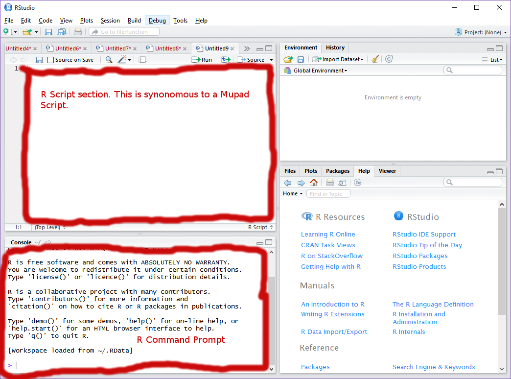
You are now ready to start using R! We will start by opening Rstudio. You’re beginning screen should look something like this:
- Workspace setup. First we will set our working directory. To do this, call the command: getwd()
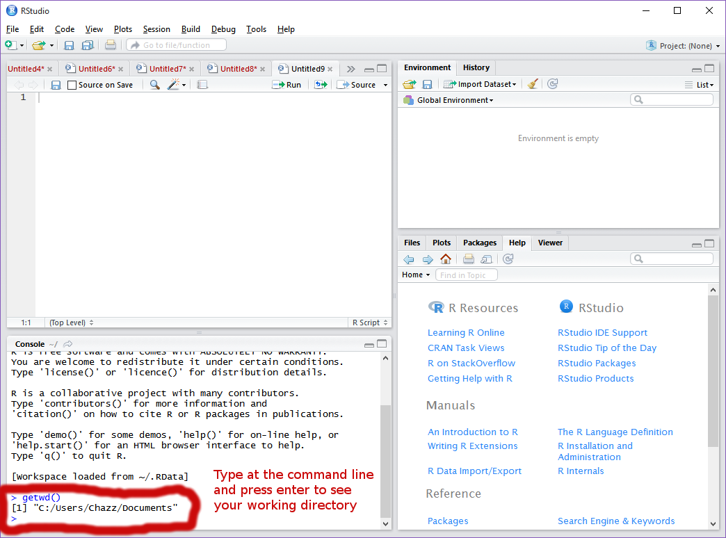
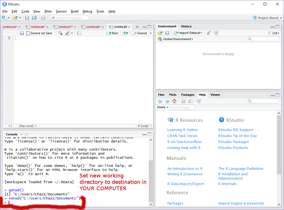
This will show to you the current folder in which you are saving your work. As is, my current folder is “Documents.” ii. This will work, but I prefer to create a folder in my documents in which I save all of my work to. We will call this folder “R.” To do this first manually create said folder in the file operator. Then, in R or R Studio, call the command:
R has its own LaTeX-like documentation format, which is used to supply comprehensive documentation, both on-line in a number of formats and in hardcopy. R web page is located at
To install R, follow the link https://cran.r-project.org/ or search CRAN within Google, and select the download for your appropriate operating system. When you use the R program it issues a prompt when it expects input commands. The default prompt is ‘>’, which on UNIX might be the same as the shell prompt, and so it may appear that nothing is happening. However, as we shall see, it is easy to change to a different R prompt if you wish. We will assume that the UNIX shell prompt is ‘$’.
In using R under UNIX, the suggested procedure for the first occasion is as follows:
Create a separate sub-directory, say work, to hold data files on which you will use R for this problem. This will be the working directory whenever you use R for this particular problem.
$ mkdir work
$ cd work
Start the R program with the command
$ R
To quit the R program the command is
> q()
At this point you will be asked whether you want to save the data from your R session. On some systems this will bring up a dialog box, and on others you will receive a text prompt to which you can respond yes, no or cancel (a single letter abbreviation will do) to save the data before quitting, quit without saving, or return to the R session. Data which is saved will be available in future R sessions.
R has an inbuilt help facility similar to the man facility of UNIX. To get more information on any specific named function, for example solve, the command is
> help(solve)
An alternative is
> ?solve
For a feature specified by special characters, the argument must be enclosed in double or single quotes, making it a “character string”: This is also necessary for a few words with syntactic meaning including if, for and function.
> help("[[")
Either form of quote mark may be used to escape the other, as in the string "It's important". Our convention is to use double quote marks for preference.
On most R installations help is available in HTML format by running
> help.start()
which will launch a Web browser that allows the help pages to be
browsed with hyperlinks. On UNIX, subsequent help requests are sent to
the HTML-based help system. The ‘Search Engine and Keywords’ link in
the page loaded by help.start() is particularly useful as it is
contains a high-level concept list which searches though available
functions. It can be a great way to get your bearings quickly and to
understand the breadth of what R has to offer.
The help.search command (alternatively ??) allows searching for help in various ways. For example,
> ??solve
Try ?help.search for details and more examples.
The examples on a help topic can normally be run by
> example(topic)
Windows versions of R have other optional help systems: use
> ?help
for further details.
Technically R is an expression language with a very simple syntax. It is case sensitive as are most UNIX based packages, so A and a are different symbols and would refer to different variables. The set of symbols which can be used in R names depends on the operating system and country within which R is being run (technically on the locale in use). Normally all alphanumeric symbols are allowed (and in some countries this includes accented letters) plus ‘.’ and ‘_’, with the restriction that a name must start with ‘.’ or a letter, and if it starts with ‘.’ the second character must not be a digit. Names are effectively unlimited in length.
Elementary commands consist of either expressions or assignments. If an expression is given as a command, it is evaluated, printed (unless specifically made invisible), and the value is lost. An assignment also evaluates an expression and passes the value to a variable but the result is not automatically printed.
Commands are separated either by a semi-colon (‘;’), or by a newline. Elementary commands can be grouped together into one compound expression by braces (‘{’ and ‘}’). Comments can be put almost3 anywhere, starting with a hashmark (‘#’), everything to the end of the line is a comment.
If a command is not complete at the end of a line, R will give a different prompt, by default
+
on second and subsequent lines and continue to read input until the command is syntactically complete. This prompt may be changed by the user. We will generally omit the continuation prompt and indicate continuation by simple indenting.
Command lines entered at the console are limited to about 4095 bytes
(not characters).
If commands are stored in an external file, say commands.R in the working directory work, they may be executed at any time in an R session with the command
> source("commands.R")
For Windows Source is also available on the File menu. The function sink,
> sink("record.lis")
will divert all subsequent output from the console to an external file, record.lis. The command
> sink()
restores it to the console once again.
The entities that R creates and manipulates are known as objects. These may be variables, arrays of numbers, character strings, functions, or more general structures built from such components.
During an R session, objects are created and stored by name (we discuss this process in the next session). The R command
> objects()
(alternatively, ls()) can be used to display the names of (most of) the objects which are currently stored within R. The collection of objects currently stored is called the workspace.
To remove objects the function rm is available:
> rm(x, y, z, ink, junk, temp, foo, bar)
All objects created during an R session can be stored permanently in a file for use in future R sessions. At the end of each R session you are given the opportunity to save all the currently available objects. If you indicate that you want to do this, the objects are written to a file called .RData in the current directory, and the command lines used in the session are saved to a file called .Rhistory.
When R is started at later time from the same directory it reloads the workspace from this file. At the same time the associated commands history is reloaded.
It is recommended that you should use separate working directories for
analyses conducted with R. It is quite common for objects with names x
and y to be created during an analysis. Names like this are often
meaningful in the context of a single analysis, but it can be quite
hard to decide what they might be when the several analyses have been
conducted in the same directory.
0.2. RStudio
RStudio is a free and open source integrated development environment (IDE) for R, a programming language for statistical computing and graphics. This is a much more user-friendly version of R that offers help in coding and displays plots and tables within the same window. To install RStudio, go to the link at https://www.rstudio.com/products/RStudio/#Desktop or search R Studio within Google and navigate into the download for your appropriate operating system. Note: You must install R before you can use R Studio
RStudio is available in two editions: RStudio Desktop, where the program is run locally as a regular desktop application; and RStudio Server, which allows accessing RStudio using a web browser while it is running on a remote Linux server. Prepackaged distributions of RStudio Desktop are available for Microsoft Windows, Mac OS X, and Linux. However, not every linux version is suitable for RStudio; there are two of them: Ubuntu 12+/Debian 8+ and Fedora 19+/RedHat 7+/ open SUSE 13+.
RStudio is written in the C++ programming language and uses the Qt framework for its graphical user interface.
The RStudio team contributes code to many R packages and projects. R users are doing some of the most innovative and important work in science, education, and industry. It’s a daily inspiration and challenge to keep up with the community and all it is accomplishing.
0.3. Basic Commands
Technically R is an expression language with a very simple syntax. It is case sensitive as are most UNIX based packages, so A and a are different symbols and would refer to different variables. The set of symbols which can be used in R names depends on the operating system and country within which R is being run (technically on the locale in use). Normally all alphanumeric symbols are allowed (and in some countries this includes accented letters) plus ‘.’ and ‘_’, with the restriction that a name must start with ‘.’ or a letter, and if it starts with ‘.’ the second character must not be a digit. Names are effectively unlimited in length.
Elementary commands consist of either expressions or assignments. If an expression is given as a command, it is evaluated, printed (unless specifically made invisible), and the value is lost. An assignment also evaluates an expression and passes the value to a variable but the result is not automatically printed.
Commands are separated either by a semi-colon (‘;’), or by a newline. Elementary commands can be grouped together into one compound expression by braces (‘{’ and ‘}’). Comments can be put almost3 anywhere, starting with a hashmark (‘#’), everything to the end of the line is a comment.
If a command is not complete at the end of a line, R will give a different prompt, by default
+
on second and subsequent lines and continue to read input until the command is syntactically complete. This prompt may be changed by the user. We will generally omit the continuation prompt and indicate continuation by simple indenting.
Command lines entered at the console are limited to about 4095 bytes
(not characters).
If commands are stored in an external file, say commands.R in the working directory work, they may be executed at any time in an R session with the command
> source("commands.R")
For Windows Source is also available on the File menu. The function sink,
> sink("record.lis")
will divert all subsequent output from the console to an external file, record.lis. The command
> sink()
restores it to the console once again.
The entities that R creates and manipulates are known as objects. These may be variables, arrays of numbers, character strings, functions, or more general structures built from such components.
During an R session, objects are created and stored by name (we discuss this process in the next session). The R command
> objects()
(alternatively, ls()) can be used to display the names of (most of) the objects which are currently stored within R. The collection of objects currently stored is called the workspace.
To remove objects the function rm is available:
> rm(x, y, z, ink, junk, temp, foo, bar)
All objects created during an R session can be stored permanently in a file for use in future R sessions. At the end of each R session you are given the opportunity to save all the currently available objects. If you indicate that you want to do this, the objects are written to a file called .RData in the current directory, and the command lines used in the session are saved to a file called .Rhistory.
When R is started at later time from the same directory it reloads the workspace from this file. At the same time the associated commands history is reloaded.
It is recommended that you should use separate working directories for
analyses conducted with R. It is quite common for objects with names x
and y to be created during an analysis. Names like this are often
meaningful in the context of a single analysis, but it can be quite
hard to decide what they might be when the several analyses have been
conducted in the same directory.
Result of last command
Last.value
In R, you can spread commands out over multiple lines, and nothing extra is necessary. R will continue reading input until the command is complete. However, this only works when the syntax makes it clear that the first line was not complete. E.g.:
 x = 3 +
4
 x = 3
+ 4
Exit the program
 q()
#  or
quit()
#.
To display a string, use
print(’hi are you doing’)
 print(’how are you doing’, quote=FALSE)
# or
print(noquote(’how are you doing’))
 print(’It\’s nice’)
#  or
print("It’s nice")
print(’Enter data:’); x=scan()
Give prompt and read character (string) input from user
x = readline(’Enter string:’)
================= to be moved to Maxima ========================
II. Reading lines
Maxima differentiates its inputs and outputs by labeling each input line with (%i#) and output line with (%o#). The output line number of your result will correspond with your input line number.
Example 0.2.1:
(%i1) 1+1;
(%o1) 2
If your output goes over a line, Maxima will put a “ / ” at the end of the line to indicate that your output will continue on the next line.
When entering commands in Maxima, you need to type “ ; ” (semicolon) and hit enter after your command line in order for your command to run. (In wxMaxima, instead of a semicolon, you need to press “ Shift + Enter ” for your command to run.)
Use “ $ ” after your command to type in more than one command.
Example 0.2.2:
(%i2) a:1$display(a);
(%o2) a = 1
done.
Keep in mind that Maxima is case sensitive when defining variables and typing commands.
Maxima follows the basic arithmetic symbols such as +(addition) -(negation) *(multiplication) /(division) ^(exponentiation) and the order of calculation.
Do not omit arithmetic symbols when typing equations. Maxima will not understand.
Example 0.2.3:
(%i3) 2x;
incorrect syntax: X is not an infix operator
Instead, type as
(%i3) 2*x;
(%o3) 2 x
Maxima follows the trigonometric expression such as sin(), cos(), tan(), asin(), acos(), atan(), sec(), csc(), cot() and the angles should be given in radian. %pi is used to indicate ![]() . Some of the common constant used by Maxima:
. Some of the common constant used by Maxima:
| %e | base of the natural logarithm (ln) |
| %i | imaginary unit |
| inf | real positive infinity |
| minf | real negative infinity |
| infinite | complex infinity |
| %phi | the golden ration (1+sqrt(5))/2 |
| %pi | 3.14159265358979323846... |
| %gamma | Euler's constant (approx 0.5772156649...) |
| false, true | boolean (logical) values |
Example 0.2.4:
(%i4) sin(%pi);
(%o4) 0
III. Simplify and Expand
expand(expr) command expands a function or an equation into a given power series
fullratsimp(expr) command finds the simplest form of an equation.
-%
Use “ % ” to refer to the most recently inputted equation.
You can use “ %on ” to refer to the output of line number n.
Example 0.3.1:
(%i10) (x+1)^3;
3
(%o10) (x + 1 )
(%i11) expand(%);
3 2
(%o11) x + 3 x + 3 x + 1
Suppose we need to organize a double summation. We can do it as
(%i11) f(x):=y(x)+sum(sum(1,i,1,j),j,1,10);
Now we use the opposite operation:
(%i12) unsum(f(x),x);
(%o12) y(x)-y(x-1)
Now we calculate modulas operations:
(%i13) mod(56,10);
(%o13) 6
(%i14) power_mod(4,15,6);
(%o14) 4
Binomial coefficient:
(%i15) binomial(10,2);
(%o15) 45